Quantitative Data Analysis and Findings

Introduction

The purpose of the current study is to assess the impact of the factors that influence the acceptance of MOOCs as a continual and progressive professional development tool within a Kuwaiti higher educational institution by professionals working in Library and Information Science (LIS) Profession. A questionnaire was administered tofor collecting the raw data from DLIS faculty members, training staff, librarians graduated from the DLIS, and librarians who work in PAAET libraries was administered. Then, Statistical Package for the Social Sciences (SPSS 22), and structural equation modeling (SEM) using Amos 22 graphics waeres employed to analyze the data.

This chapter aims to present the analysis and the research findings of the quantitative data of the study. Descriptive statistics such as frequencies and averages areis used to explore the samples’ features and characteristics. Subsequently, the main data analysis and assessing model fit is provided. Moreover, in the latent factors process of analysis, two steps are applied and performed by the researcher: firstly, a confirmatory factor analysis (CFA) to assess and validate the measurement model followed by validity and reliability; secondly, assesse the (SEM) in terms of overall goodness of fit in order to ultimately test the research hypothesis.

Organization of data

The questionnaire included 26 questions. The 26 questions are subdivided into three sets: demographic variables, closed questions and open ones. The content of the questions was designed according to the UTAUT model’s originality combined with new factor analysis: Firstly, experience of internet and online communications, general knowledge, current methods of professionals, and motivator/inhibitor concepts for professional development; secondly, MOOC perceptions and effects; thirdly, collection of demographic details.

Pilot Study

As fFive respondents are the minimum for a questionnaire’s validity (Francis et al., 2004), so a pilot of 16 was selected from LIS professionals, including: academic librarians and academic faculty members. This process revised the design for improvement prior to actual fieldwork (Grossnickle & Raskin, 2001), although the assessments indicated that no issues were present. Nevertheless, the questions’ wording and expression were altered to function with the participants’ feedback.

Total Sample and collecting data processes

The sample size is based on a number of factors that relate to the complexity of the model, and anticipated rates of missing data or estimations that can direct the researcher, although large samples normally produce general stability (Hair et al., 2006). Sampling incorporates case number selection to evaluate the selection process for: population, frame, method, size and selection (Seawright and Gerring, 2008; Sekaran, 2000; Zikmund, 1999).

A cover letter was emailed to participants in order to detail the research objectives, questions, and intent, as well as the researcher’s contact details, together with the online questionnaire’s link. The invitation was structured through various ways. First, the PAAET graduates' office was contacted for assistance in reaching the DLIS graduates, and circulating the email. Second, PAAET Academic library managers were asked permission in accessing academic librarians, and in circulating the email. Third, the head of the Library & information association was contacted to circulate the questionnaire among LIS professionals who graduate from DLIS. Fourth, different LIS professional peers were contacted to invite participation. Fifth, the email list of LIS professionals was ascertained. Sixth, the head of the library and science department was contacted to invite participation and circulation of the questionnaire. Lastly, Twitter and Facebook were used in line with promoting the study.

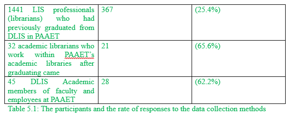
The overall response comprised of 416 participants. From LIS professionals, who graduated from DLIS in PAAET 388 responded, response rate of 26.92% was seen. Academic librarians who had graduated from DLIS and worked at PAAET equaled 21 responses, at a very good rate of 65.6%. The response was 28 for Academic faculty members & staff at PAAET, with a very good response rate of 62.22%.

Overall, the recipients of the questionnaire totaled 1518. Firstly, LIS professionals (librarians) who had previously graduated from DLIS in PAAET equaled 1441, with a response rate of 367 responses (25.4%), which is considered good. Secondly, academic librarians who work within PAAET’s academic libraries after graduating came to 32, with a response rate of 21 (65.6%), which is also considered good. Thirdly, DLIS Academic members of faculty and employees at PAAET equaled 45, with a response rate of 28 (62.2%), which is also good (see table 5.1). The questionnaire respondents were made up of 416 males and females, including DLIS graduates, Academic librarians who graduated from DLIS and were working at PAAET, and DLIS Academic faculty members & staff members working at PAAET. In order to illustrate the distribution of respondents’ frequency tables (numbers and percentages) were used. SurveyMonkey was used for distributing the survey, which converts the gathered data to SPSS. SPSS 22 and AMOS 22 were used to analyse this data. From the table below it can be seen that the participants were from different fields, and this shows that the researcher has tried to avoid biasness by selected different kinds of respondents.

Participants Characteristics and Descriptive Statistics

Hair et al (2006) claim that descriptive statistics enable the researcher’s understanding of the studied data. Furthermore, the findings of descriptive analysis can be administered to facilitate the discussion of the results that developed from other advanced statistical approaches (Malhotra, 2010). Descriptive analysis was used to determine all measurement items of the current study including frequencies, means and standard deviations.

Participants’ Demographic Profile

The focus of the study is on professionals of LIS who graduated from DLIS, including PAAET academic librarians (93.2), together with DLIS academic faculty members and employees at PAAET (6.73%). Most respondents in the sample were young adults (21- 31) or (37.02%), with ages be 31-40 comprising 35.10%, as technology is believe to be more accepted by these two age groups. The ages of 41-50 showed 19.23% of respondents, with those of 51-60 comprising 7.93% and only 0.72% for plus 60 years. 55.53 % of the respondents were female, with males at 44.47%, which is a direct representation of the population in Kuwait (Chapter 1, Section 3.4.4, Population), alongside women preferring LIS (Moreiro, 2001). Indeed, between 1991-2015, 873 females and 568 males have graduated from DLIS. A detailed demographic profile of the respondents is presented in table 5.2 below.

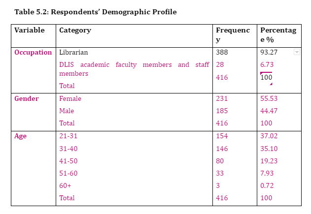
The table above also shows the varied descriptive statistics of the respondents. This clearly shows that the research has tried to conduct the research in an ethical manner by avoiding any kind of biasness and giving an equal chance to all the individual of the population.

Participants’ Continuing professional Development Current situation

Using MULT Response Analysis helps to answer question one: “How do LIS professionals currently continue and progress their professional development and what might motivate or inhibit them?” . In the process of survey question analysis that formulates from a variety of answers, it is possible to conduct a frequency analysis, which generates descriptive statistics for each chosen option, and as a consequence, the researcher is finally presented with the amount of respondents who have chosen that specific option (Schaeffer and Dykema, 2011; Robert, 2006). Therefore, each respondent in the questionnaire was asked to choose what directly applied to them, or state another method which was not mentioned in the questionnaire.

It a known fact that different people have different needs and desires, and on the basis of individual needs and desire, an organisation needs to design its employee motivation and development plans. That is, it is essential for the institute to devise customised strategies for all the employees. The table above shows that the organisation has used several techniques for the continuing profession development of its employee. It means, the institute ensures that all the employees are developing and growing with the organisation as the institute is provided customised development opportunities to its employees.

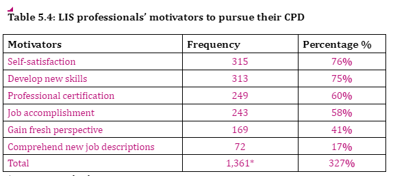
* N = 416, multiple response.

Motivational factors to pursue CPD were identified through 6 options: Self-satisfaction and developing new skills, gaining professional certification, accomplishing work tasks, gingain gaining fresh perspective, and attempting to comprehend new job descriptions. Self-satisfaction and developing new skills were the highest recorded, at 75% and 76% respectively,. wWhile, attempting to comprehend new job descriptions was the lowest at 17%. Furthermore, other factors (1%) were noted, such as: filling of skills gap, and career development,

* N = 416, multiple response.

Respondents were also asked state what barriers prevented their pursuit of CPD. A lack of time was the highest at 71% due to family or personal commitments, with location of the course or event (61%), as traffic congestion within Kuwait can cause problems. The two lowest factors were timing of the course or event and duration of the course or event (46% and 24% respectively). Nevertheless, laziness was described as the barrier by a solitary respondent.

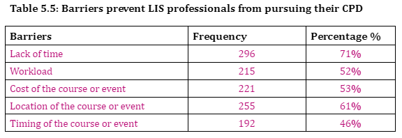
* N = 416, multiple response

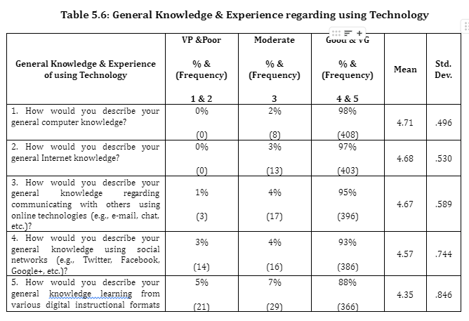
Participants’ General Knowledge & Experience of the Internet & Online communication

General knowledge and experience of the Internet, technology, and online communication was ascertained. To obtain the frequency and mean, standard deviation, as well as responses from participant a statistical summary was applied, where they rated themselves on a Likert scale (1=Very Poor, 2=Poor, 3=Moderate, 4=GOOD, 5=Very Good), see table 5.6 below. Furthermore, the overall feedback was conjoined between the answers, as cultural understanding in Kuwait does not clarify distinguish between: poor-very poor, or good-very good.

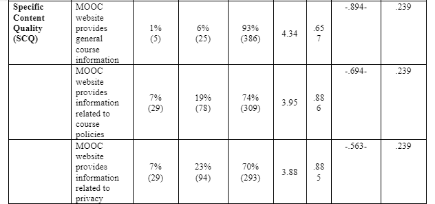
Constructs correlation to MOOC

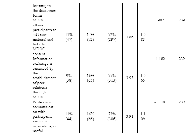
The questionnaire highlighted a set of expectations and constructs formed derived from the literature review. To obtain the frequency and mean, standard deviation, as well as responses from participant, a statistical summary was applied, where they rated themselves on a Likert scale (1= strongly disagree, 2= disagree, 3=neutral, 4= agree, 5= strongly agree) as a measuring rates of their acceptance of MOOC as a tool of CPD, see table 5.7 below.

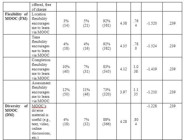
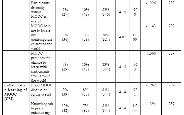
Data Normality

Data normality describes the distribution of the individual measurement items of the study variables that could be tested by evaluating Skewness and Kurtosis values. Skewness is used when the frequency distribution of the data does not fit as symmetrical distribution. Whereas, Kurtosis reveals the extent of which flattening or peaking in the frequency distribution of the data is beyond the normal distribution (Katz, Elmore and Wild, 2014; Collis & Hussey, 2009). Ordinal variables with 5 or more categories, such as 5-point Likert-type scales of agreement, can be safely treated as “continuous”, (Finney & DiStefano 2013). To determine whether data is normally distributed, univariate distribution is examined using skewness and kurtosis. There is no concern about normality violation if skewness <2 and kurtosis < 7 (Kim, 2014; West, Finch, & Curran, 1995). Kurtosis is usually a greater concern than skewness. The absolute values of resulting skewness and kurtosis for all items of constructs given in pervious table (5.7) were less than the thresholds (skewness <2 and kurtosis < 7), and hence data was normally distributed.

Main Statistical Data Analysis

In order to define and model the intricate connection that exists between multiple dependent and independent constructs, SEM has been utilised (Kline, 2005). Indeed, the utilisation of SEM in the areas of behavioural sciences and IT/IS research are strongly recommended as beneficial (Ambak, et. al. 2011; Gefen et al., 2000). Furthermore, the current study has implemented a two-step approach that Anderson & Gerbing (1988) theorised as recommendable. Firstly, in order to examine reliability and validity the measurement model is assessed. Secondly, the structural model is assessed in order to test the hypotheses in the research and the model’s suitability.

In comparison to the one step approach, the two-step approach is advantageous, as beneficial construct measurements are assured, which are represented in the valid structural Equation model (Hair et al., 2006). What is more, a measurement model is included in the two-step approach, which is followed by the structural Equation model (Schumacker & Lomax, 2004). Overall, the structural Equation model defines the connections that exist among latent variables as theorised, while the measurement model specifies the relationships that among measured/observed variables that underlie the latent variables. In addition, the structural model provides an assessment of nomological validity is provided by the structural model, while an assessment of convergence and discriminant validity is provided by the measurement model.

Assessing Model Fit

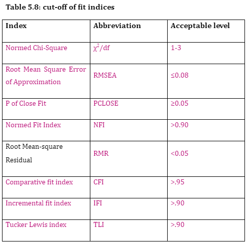
In order to assess a model’s fit, goodness-of-fit indices (GOF) need to be inspected. GOF indices reveal the degree of which the observed and estimated covariance metricesmatrices are related and the closer values of the observed covariance metrices matrices and estimated ones suggest a better model fit (Hair et al., 2006). Thus, the observed and estimated covariance matrices will be identical in a perfect research theory. Further, a researcher should address multiple indices revealing different types of GOF because it is difficult to determine whether a model has a good or poor model fit across all situations using goodness of fit indices (Hair et al., 2006). There are different indices introduced in order to assess goodness-of-fit such as absolute fit indices, and incremental indices fit indices (Kline, 2011). These two types of indices were used in the current study: absolute fit indices (such as: χ2/df, RMSEA, and PCLOSE, RMR), incremental indices (such as: NFI, CFI, IFI, TLI).

Absolute Indices

To assess the fitted model in CFA, which presents the minimum discrepancy between the covariance matrix of data and implied model, χ2/df (CMIN/DF) test is used (Holmes-Smith, 2011). The acceptable level of χ2/df ranges from 1 to 3 (Hair et al., 2010).

Separately, Root Mean Square Error of Approximation (RMSEA) is a measure to assess model fit (Hair et al., 2010); this functions in terms of adequate sensitivity to model misspecification (Byrne, 2010). If RMSEA is > .05 but < .08 ", then it could be a reasonable approximate fit (Kline, 2005). In contrast, even when RMSEA is less than 0.05 and the resulting p-value of RMSEA (PCLOSE) is less than 0.05 then the mean value of RMSEA can be ascertained. On the other hand, if the p-value is more than 0.05 it is a close fit to the hypothesis. Root Mean-square Residual (RMR) is used to calculate the average difference between the variance-covariance matrix for the hypothesised model and the variance-covariance of the sample, where RMR<.05 (Byrne, 2010).

Incremental Fit Indices

These types of indices are based on a comparison of the fitted model with the baseline model, which is the null model (independence model), where there are no correlations between the measured variables. The value of incremental indices ranges from 0.0 and 1.0, where zero means that fitted models are better than the null model, whilst 1.0 indicates that the model is a perfect fit (Holmes-Smith, 2011). Normed Fit Index (NFI) is indicator of Incremental Fit , (Holmes-Smith, 2011). Moreover, comparative fit index (CFI) is another indicator which is insensitive to model complexity (Hair et al., 2006). In addition, incremental fit index (IFI), which is also known as Bollen's IFI reintroduces the scaling factor so that the IFI values range between 0 and 1with higher values indicating a better fit to the data (Kelloway, 2014). Likewise, Tucker Lewis index (TLI), which is sometimes known as non-normed fit index (NNFI), is similar to the NFI. However, the TLI is lower, and hence the model can be considered as less acceptable, if the model is complex (Holmes-Smith, 2011). The cut-off levels of fit indices considered in this study are provided in Table 5.8.

According to Hair et al. (2010) reporting three to four fit measures would be sufficient enough to prove a model’s fit. In this study, eight fit indices representing two different kinds of goodness of fit along with Chi-Square and the associated degree of freedom and significance value were reported in order to conclude the model’s fit.

Measurement Model

Using CFA, the researcher will be able to assess the items validity for measuring the constructs using the number of indices (Awang, 2015; Hair et al. 2006) which were detailed previously. For each two items, the covariance between their corresponding errors is examined to drop any items with high variance (Byrne, 2001; Hair et al., 2006). Also, low multiple correlation is to be monitored to assess the items contribution. CFA is to be used for determining the order of underlying model, namely first or higher order models (Marsh, 1985). In following, the assessment of the constructs is demonstrated.

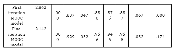
The fourteen constructs included in the initial overall measurement model measured by 54 items was subjected to confirmatory factor analysis (CFA). The CFA finding demonstrated rather poor model fit (CMIN/df = 2.842, NFI = .837, RMR = .047, IFI = .888, TLI = .857, CFI = .887, RMSEA = .067, PCLOSE = .000). When these values are compared with the cut-off of fit indices, it can be seen that for some of the test, the result is not meeting acceptable level required. Therefore, some modifications in the model are needed in order to create a model that better fit the data.

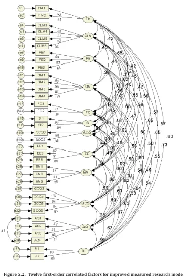
Figure 5.1: fourteen first-order correlated factors for improved measured research model

Measurement Model Improvement

By using fourteen one-order factors, the full model that consists of exogenous and endogenous constructs is provided in Figure 5.1. Moreover, the resulting indices that are given in Table 5.8 confirmed that the fourteen first-order correlated factors’ measurement model produced good indicators for fitting the full model. Hence, since the results showed that the fit of measured model is good, no re-speciation is required.

The model fit indicators were under the acceptable threshold. Two iterations were conducted to eliminate non-significant items in measuring the structures of MOOC, and to improve the indicators of model fit. The Standardized Residual Covariances, which show the discrepancy between variables, should be less than two in absolute (Joreskog & Sorbom, 1984). Standardised residual covariances should not be above 2.58 or below - 2.58 -what is known as the absolute value 2.58 (Pedhazur and Schmelkin, 2013; Byrne, 2001), and Modification indices (MI) showing high covariance between residuals accompanied by high regression weights between these residuals’ construct are candidate for deletion (Byrne, 2001; Hair et al., 2006). High covariance were detected between several items as follows:

1. BI2 showed a high standardized residual covariance value with SI, OM4 and CLM.
2. TQ6 had a high standardized residual covariance value with TQ5, FM, FM2, OM1, SI1 and SI2.
3. TQ5 had a high standardized residual covariance value with FM1, FM2 and SI2.
4. TQ4 had a high standardized residual covariance value with GCQ2, OM3, OM1, OM2 and PE3.
5. Also, TQ3 had a very high standardized residual covariance value with SCQ1.
6. FM4 showed a very high standardized residual covariance value with DM4, DM3, DM3, DM1, CLM1, BI3, AQ4, AQ1, CLM6, CLM5, CLM3, CLM2
7. Also, FM3 showed a very high standardized residual covariance value with DM4, DM3, DM1, CLM1, BI1, AQ4, AQ1, EE1 and OM4
8. The item TQ2 showed high standardized residual covariance value with SCQ1.
9. TQ1 showed a high standardized residual covariance value with GCQ1, SCQ1 and SI2.
10. The item DM4, showed a high standardized residual covariance value with SCQ1, SI1 and OM4.
11. Also, DM3 showed a high standardized residual covariance value with SI1.
12. DM1 showed a high standardized residual covariance value with SI2 and SI1
13. DM2 showed a high standardized residual covariance value with OM4 and SCQ1.
14. FC3 showed a high standardized residual covariance value with SCQ2, SI2 and SI1.
15. SCQ1 showed a high standardized residual covariance value with AQ3, AQ4, GCQ3, EE2 and EE1.
16. The item GCQ2 showed a high standardized residual covariance value with OM2.
17. GCQ1 showed high covariance value with GCQ2 and PE3.
18. CLM1 showed high standardized residual covariance value with BI1, OM4, OM3, OM2, FM2 and FM1.
19. CLM2 showed high standardized residual covariance value with BI1, BI3, GCQ3, OM4 and OM3.

Items that demonstrated high covariance were deleted to improve the model fit indices (Byrne, 2001). Based on that, the following items: BI2, TQ6, TQ5, TQ4, TQ3, TQ2, TQ1, FM4, FM3, DM4, DM3, DM2, DM1, FC3, SCQ1, GCQ2, GCQ1, CLM1, and CLM2 were deleted.

After the deletion of those items, a re-run of CFA resulted in the following model fit indexes: CMIN/df = 2.142; NFI =.929; CFI =.955; RMR=.032; IFI=.956; TLI=.946 and RMSEA = .052 with PCLOSE=.174, (see Table 5.9). Since the model fit indices have been improved and were within acceptable criteria according to cited indices, the next stage is to examine the validity and reliability of the model, (see Figure 5.2).

Validity

Measurement validity is considered to be a critical concern in social research. Measurement validity is defined by Neuman (2006) to meanas “how well the conceptual and operational definitions match each other” (p. 192). Examining the measurement model gives indicators to assess convergent and discriminant validity, which indicate nomological validity (Schumacker & Lomax, 2004).

Unidimensionality

Unidimensionality is the degree to which items loading only on their respective constructs without having “parallel correlational pattern(s)” (Segars, 1997). Nunnally (1978) declared the necessity of examining the unidimensionality of each construct incorporated in the conceptual model as prerequisite step for validity and reliability tests. Unidimensionality is achieved when all measuring items have acceptable factor loadings for the respective latent construct. In order to ensure unidimensionality of a measurement mode, unidimensionality also requires all factor loadings to be positive and the factor loading for every item should exceed 0.5 ( Bin and Afthanorhan, 2014; Zainudin, 2010; Segars,1997). Table 5.11 showed that all the items had positive loading and exceeded 0.5.

Discriminant Validity

“Discriminant validity is considered a key measure to test the instrument because ‘without it researchers cannot be certain whether results confirming hypothesized structural paths are real or whether they are a result of statistical discrepancies” (Farrell, 2010, p. 324). Discriminant validity is supported if the square root of average variance extracted of each construct is more than its correlation with other constructs (Guo et al., 2011). Table 5.10 showed that the results achieved a satisfactory level of discriminant validity.

Table 5.10: Inter-correlation Matrix for discriminant validity

The inter-correlation matrix shows that there exist moderate to strong positive association between all the variables. This means, with the increase in any of the variable, there will be increase in the others variables as well and vice-versa.

Convergent Validity

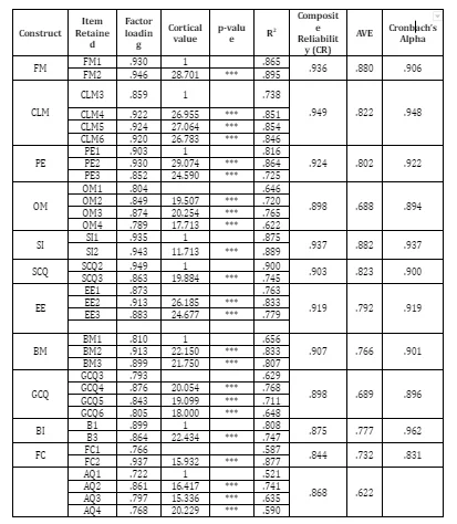
Convergent validity is an important aspect to assess the constructs. It evaluates relationships between the observed variables and the constructs (Schumacker & Lomax, 2004). According to Hair et al. (2006) the term convergent validity specifies the degree to which the items of a particular construct converge or share a high proportion of variance in common. Factor loading, variance extracted and composite reliability can be used to assess convergent validity. The resulting loading is used to assess the convergent validity, and this type of validity is achieved when each item loading in the construct exceed 0.50 in order to achieve convergent validity (Gefen & Straub, 2005; Hair et al., 2006; Holmes-Smith, 2011; Aggelidis & Chatzoglou, 2012; Sun & Teng, 2012). The validity can be achieved if the value of factor loading is significantly different from zero using critical ratio (Holmes-Smith, 2011). The values of resulting factor loading that is shown in Table 5.11 for the majority of items used in the current study were more than .80, which confirms the validity of the constructs. Moreover all the items were very highly significant. The convergent validity could also be verified by computing the Average Variance Extracted (AVE) for every construct. The value of AVE should be 0.5 or higher for this validity to achieve (Holmes-Smith, 2011). Based on the results given in Table 5.11, the AVE was higher than 0.70 for all the items. The lowest AVE was seen for GCQ where the AVE was .689, but since this value is close to 0.70 and corresponding loadings were higher than 0.50 and very highly significant, the convergent validity of GCQ was supported.

Moreover, table below also shows that the data collected for the research is highly reliable. The Cronbach’s Alpha value for each construct is more than 0.80, it shows that the collected data is highly reliable and will result in valid result that can be generalised under various situations.

Table 5.11: Validity and reliability for measured model

Reliability

Reliability refers to consistency of measurement (Neuman, 2006). Leedy and Ormrod define reliability as: “the consistency with which a measuring instrument yields a certain result when the entity being measured hasn’t changed” (2010, p. 29). The indicators to measure reliability used in this study are explained next: Squared Multiple Correlation (SMC) ‘item reliability’; Cronbach's alpha; Coefficient H; Construct Reliability (composite reliability) (CR). These are explained in the following sections.

Squared Multiple Correlation (SMC) ‘item reliability’

The squared multiple correlation coefficient represented the amount of variance of one variable explained by the other observed variables (Schumacker & Lomax, 2004). It will be used to measure the reliability of each item (Bagozzi & Yi, 2012). If SMC exceed 0.50, then the observed item has a good reliability, and also 0.30 is considered as an acceptable level (Holmes, 2011). Table 5.4 shows the SMC for each item. All the items exceeded 0.50. Therefore, based on the value of SMC, all the items given in the table were used to measure the constructs of the model are reliable.

Construct reliability (composite reliability)

Construct reliability (CR) is used to measure the reliability of all the observed variables that represent the construct, in order to examine the internal consistency of the measures (Holmes-Smith, 2011). A value of construct reliability less than 0.70 can be acceptable (Bagozzi & Yi, 2012). From 5.11, the resulting CR for all the items were higher than 0.70 indicating that the constructs of the model are reliable.

Cronbach's alpha

Cronbach’s alpha is computed for measuring an internal consistency so that reliability for each construct model is obtained (George & Mallery, 2012). George and Mallery (2012) suggested a rule of thumb for Cronbach's alpha: α > 0.9 – excellent; α > 0.8 – good; α > 0.7 – acceptable; α > 0.6 – questionable; α > 0.5 – poor; and α < 0.5 – unacceptable. From Table 5.11, Cronbach’s alpha ranged from good (>0.80) to excellent (>0.90), which indicated that the resulting model reliability was very satisfying.

Test of the Hypotheses

The model was designed in order to assess the relationships between the fourteen constructs using SEM (See Figure 5.2). Following this, it is necessary to test the effect of the moderating variables: gender, age and general knowledge & experience of the internet on the model. The fitted without moderating variables was referred to as the “basic MOOC model”.

Research Model

According to Cohen (1988) and Sridharan et al. (2010), the standardised values of regression coefficient are classified into the following strength classes: 0.2 (low); between 0.2 and 0.5 (moderate); and more than 0.5 (strong). Table 5.12, for the significant effects, the CLM showed the higher contribution towards BI compared with other variables. Then, it was followed by BM, FM, SCQ, FC, OM and SI. In contrast, for nonsignificant effects, PE and EE showed very low contributions.

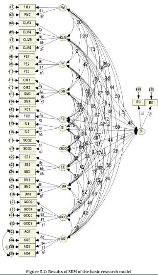
As shown in Table 5.12, the effect of CLM on BI was found to be positive and significant (β=.347, p-value=.000), and hence, “BI was positively related to the CLM”. Moreover, The FM led significantly to increase in the BI attitude (β=.208, p-value=.000), and hence, “BI was positively related to FM”. The PE showed positive and significant effects on BI (β=.092, p-value=.061), and as a result “BI was positively related to the PE”. The SCQ showed positive effect on BI (β=.086, p-value=.042), and as a result “BI was positively related to the SCQ. The SI showed negative effect on BI (β=-.113, p-value=.003), and as a result “BI was negatively related to the SI. The OM led significantly to decrease in the BI attitude (β=-.178, p-value=.025), and hence, “OM was negatively related to FM”. The FC led significantly to increase in the BI attitude (β=.237, p-value=.002), and hence, “BI was positively related to FC”. The BM led significantly to increase in the BI attitude (β=.209, p-value=.000), and hence, “BI was positively related to BM”. The rest of variables: EE showed positive influence, but it was statistically not significant. Similarly, GCQ and AQ seemed to have positive influence on BI, but there were not significanthet effect on BI was insignificant.

Notes: *** p-value < 0.01 (very highly significant); ** p-value < 0.05 (highly significant) ; * p-value < 0.10 (significant)

Moderation of General Knowledge & Experience of the Internet (GKE)

The significant p value (<.05) for z-score indicates that the structural weights are not similar between the two groups, and there is moderation effect. Namely, significant changes indicate that there are non-equivalent paths (Hair et al., 2006).

This model is quite useful in determining the impact of one variable on the others. As per the model, if the p-value or the significance value is less than 0.05, it means there is no significant impact of one variable over another. On the other hand, if the p-value or the significance value is more than 0.05, it shows there is significant of one variable over others.

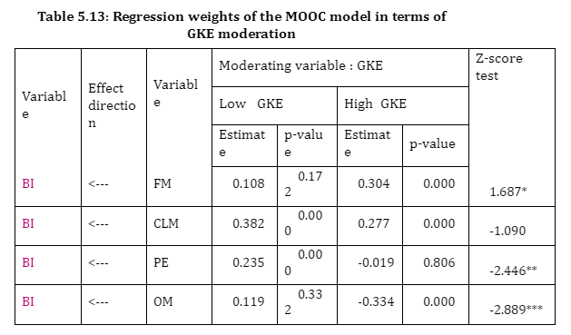
Table 5.13 showed that low and high GKE seemed to be positively affected by CLM when forming attitudes toward BI (βlow = 0.383, p-value= .000; βhigh = 0.277, p-value= .000). GKE was not moderation variable for CLM (z-score=-1.090).

Only, high GKE group tended to be positively affected by FM when forming attitudes toward BI (βlow = 0.108, p-value= .172; βhigh = 0.304, p-value= .000). As a result, GKE was moderation variable for FM (z-score=1.687*).

Additionally, only high GKE seemed to be positively affected by BM when forming attitudes toward BI (βlow = 0.068, p-value= .310; βhigh = 0.263, p-value= .070). However, GKE was not moderation variable for BM (z-score=1.222).

Only low GKE was positively affected by PE when forming attitudes toward BI (βlow = 0.235, p-value= .000; βhigh = -0.019, p-value= .806). As a result, GKE was moderation variable for PE (z-score=-2.446**).

Only high GKE tended to be positively affected by SCQ when forming attitudes toward BI (βlow = 0.064, p-value= .200; βhigh = 0.212, p-value= .015). However, GKE was moderation variable for SCQ (z-score=1.467).

High GKE was positively affected by EE when forming attitudes toward BI, whilst low GKE showed negative effect (βlow = -0.144, p-value= .083; βhigh = 0.201, p-value= .070). As a result, GKE was moderation variable for EE (z-score=-2.486**).

Low GKE was negatively affected by SI when forming attitudes toward BI (βlow =-0.100, p-value= .022; βhigh = -0.043, p-value= .544). GKE was not moderation variable for SI (z-score=-0.678).

Only high GKE was positively affected by OM when forming attitudes toward BI (βlow = 0.119, p-value= .332; βhigh = -0.334, p-value= .000). As a result, GKE was moderation variable for OM (z-score=-2.889***).

FC showed significant positive effect on BI for low GKE (βlow = 0.252, p-value= .028; βhigh = -0.084, p-value= .421). GKE was not moderation variable for FC (z=-1.079).

GCQ showed insignificant negative effect on BI for low GKE, but it was insignificant positive influence for high GKE. AQ showed insignificant positive effect on BI for both groups of GKE.

Thus for low GKE; CLM, PE, FC and SI have significant positive impact on BI as the p-value or the significance value of these variables is less than 0.05. On the other hand, for high GKE; FM, CLM, OM and SCQ have significant positive impact on BI as the p-value or the significance value of these variables is less than 0.05.

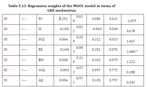
Notes: *** p-value < 0.01; ** p-value < 0.05; * p-value < 0.10

Moderation of Gender

Table 5.14 showed the estimated regression coefficients for the research model. Females and males seemed to be positively affected by CLM when forming attitudes toward BI (βmale =.493, p-value= .037; βfemales = 0.205, p-value= .006). Gender was not moderation variable for CLM (z-score=-.155).

Only males were likely to be positively affected by SCQ when forming attitudes toward BI (βfemale = .032, p-value= .590; βmale = .258, p-value= .007). As a result, gender was moderation variable for SCQ (z-score2.567**).

Only males were likely to be positively affected by PE when forming attitudes toward BI (βfemale = -.027, p-value= .710; βmale = .154, p-value= .037). As a result, gender was moderation variable for PE (z-score=-1.744**).

Only females were likely to be positively affected by SI when forming attitudes toward BI (βfemale = -.219, p-value= .000; βmale = -.062, p-value= .263). As a result, gender was moderation variable for SI (z-score=2.029**).

Only females were likely to be positively affected by AQ when forming attitudes toward BI (βfemale = .234, p-value= .037; βmale = -.512, p-value= .177). As a result, gender was moderation variable for AQ (z-score=1.888*).

Females and males were likely to be negatively affected by FM when forming attitudes toward BI (βfemale = 0.205, p-value= .006; βmale =- 0.187, p-value= .037). Gender was not moderation variable for FM (z-score=0.155).

Only females were likely to be positively affected by FC when forming attitudes toward BI (βfemale = 0.494, p-value= .001; βmale = .195, p-value= .118). However, gender was not moderation variable for FC (z-score=1.517).

Females and males were likely to be positively affected by BM when forming attitudes toward BI (βfemale = 203, p-value= .000; βmale = .369, p-value= .027). Gender was not moderation variable for BM (z-score=-.946).

OM had significant negative effect on BI for female, but it was insignificant negative influence for female (βfemale = -.208, p-value= .074; βmale = -0.093, p-value= 0.495). Gender was not moderation variable for OM (z-score=0.645).

GCQ showed significant positive effect on BI for male, but it was insignificant positive influence for female (βmale = 0.353, p-value= 0.058; βfemale = 0.041, p-value= 0.772). Statistically, gender was not moderation variable for GCQ (z=-1.330).

EE showed insignificant negative effect on BI for males and females, and hence gender was not moderation variable for EE.

Thus, in case of males, FM, CLM, PE, SCQ and BM have significant positive impact on BI as the p-value or the significance value of these variables is less than 0.05. On the other hand, for females; FM, CLM, FC, SI, BM and AQ have significant positive impact on BI as the p-value or the significance value of these variables is less than 0.05.

Table 5.14: Regression weights of the MOOC model in terms of gender moderation

Notes: *** p-value < 0.01; ** p-value < 0.05; * p-value < 0.10

Moderation of Age

Table 5.15 showed the estimated regression coefficients for the research model. Both age groups seemed to be positively affected by CLM when forming attitudes toward BI (β<=30 = 0.236, p-value= .001; β>30 = 0.366, p-value= .000). As a result, age was not moderation variable for CLM (z-score=1.424)

Table 5.15 showed the estimated regression coefficients for the research model. Both age groups seemed to be positively affected by CLM when forming attitudes toward BI (β<=30 = 0.236, p-value= .001; β>30 = 0.366, p-value= .000). As a result, age was not moderation variable for CLM (z-score=1.424)

Ages of >30 tended to be negatively affected by SI when forming attitudes toward BI (β<=30= -0.092, p-value= .097; β>30 = -.105, p-value= .034). As a result, age was not moderation variable for SI (z-score=-.172).

Moreover, both age groups seemed to be positively affected by FM when forming attitudes toward BI (β<=30 = 0.214, p-value= .027; β>30 = 0.230, p-value= .000). As a result, age was not moderation variable for FM (z-score=-.136)

Only ages of <=30 tended to be positively affected by PE when forming attitudes toward BI (β<=30= 0.167, p-value= .070; β>30 = 0.036, p-value= .540). The age was not moderation variable for PE (z-score=-1.194)

Only age groups of >30 tended to be positively affected effect by BM when forming attitudes toward BI (β<=30 = 0.112, p-value= .128; β>30 = 0.273, p-value= .000). The age was not moderation variable for BM (z-score=1.469)

Ages of >30 tended to be positively affected by FC when forming attitudes toward BI (β<=30=0.132, p-value= .390; β>30 = 0.266, p-value= .003). However, age was not moderation variable for FC (z-score=.752).

SCQ showed insignificant positive effect on BI for age<=30 years but it showed significant positive effect on BI for age>30years (β<=30=0.047, p-value= 0.484; β>30 = 0.126, p-value= .048). Statistically, age was not moderation variable for SCQ (z=.850)

OM showed significant negative effect on BI for high age group (β<=30=-0.205, p-value= 0.279; β>30 = -0.176, p-value= .051). Statistically, age was not moderation variable for OM (z=1.36).

OM showed significant negative effect on BI for high age group (β<=30=-0.205, p-value= 0.279; β>30 = -0.176, p-value= .051). Statistically, age was not moderation variable for OM (z=1.36).

EE showed insignificant negative effect on BI for age>30 years but insignificant positive effect on BI for age<=30years. Age was not moderation variable for EE.

Thus, in case of age <= 30 years, FM, CLM and GCQ have significant positive impact on BI as the p-value or the significance value of these variables is less than 0.05. On the other hand, for age > 30 years; FM, CLM, FC, SI, SCQ and BM have significant positive impact on BI as the p-value or the significance value of these variables is less than 0.05

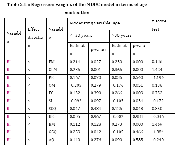
Notes: *** p-value < 0.01; ** p-value < 0.05; * p-value < 0.10

Result of Hypothesis

The hypothesis (H1), which states that performance expectancy (PE) positively influences attitude toward using behavioural intention, was accepted.

1. GKE led to a significant moderating effect between relationships, where only low GKE was positively affected by PE when forming attitudes toward BI.
2. Gender led to significant moderating effects between relationships, where male tended to be positively affected by PE when forming attitudes toward BI.
3. Age did not lead to significant moderating effects between relationships.

The hypothesis (H2), which states that effort expectancy (EE) which positively influences attitudes toward behavioural intention, was rejected.

1. . GKE led to significant moderating effects between relationships, where high GKE was positively affected by EE when forming attitudes toward BI, whilst low GKE showed negative effect.
2. Gender did not lead to significant moderating effects between relationships.
3. Age did not lead to significant moderating effects between relationships.

The hypothesis (H3), whicch states that social influence (SI) which positively impacts upon attitudes toward behavioural intention, was rejected.

1. GKE did not lead to significant moderating effects between relationships.
2. Gender led to significant moderating effects between relationships, where only female were likely to be positively affected by SI when forming attitudes toward BI.
3. Age did not lead to significant moderating effects between relationships.

The hypothesis (H4), which states that facilitating conditions (FC) which positively influence attitudes toward behavioural intention, was accepted, where there is significant effect.

1. GKE did not lead to significant moderating effects between relationships.
2. Gender did not lead to significant moderating effects between relationships.
3. Age did not led to significant moderating effects between relationships.

The hypothesis (H6), which states that general content quality (GCQ) which positively influences on attitudes toward behavioural intention, is rejected, where there is no significant effect.

1. GKE did not lead to significant moderating effects between relationships.
2. Gender did not lead to significant moderating effects between relationships.
3. Age led to significant moderating effects between relationships, where only ages of <=30 tended to be positively affected by GCQ when forming attitudes toward BI.

The hypothesis (H7), which states that specific content quality (SCQ) which positively influences upon attitudes toward behavioural intention, was accepted, where there are significant effects.

1. GKE lead to significant moderating effects between relationships, where only high GKE tended to be positively affected by SCQ, when forming attitudes toward BI.
2. Gender led to significant moderating effects between relationships, where only males were likely to be positively affected by SCQ when forming attitudes toward BI.
3. Age did not lead to significant moderating effects between relationships.

The hypothesis (H8), which states that appearance quality (AQ) which positively influences upon attitude toward behavioural intention, is rejected, where there are no significant effects.

1. GKE did not lead to significant moderating effects between relationships.
2. Gender led to significant moderating effects between relationships, where only female were likely to be positively affected by AQ when forming attitudes toward BI.
3. Age did not lead to significant moderating effects between relationships.

The hypothesis (H9), which states that openness of MOOC (OM) whichpositively influences upon attitudes toward behavioural intention, was rejected.

1. GKE led to significant moderating effects between relationships where only high GKE was positively affected by OM when forming attitudes toward BI.
2. Gender did not lead to significant moderating effects between relationships.
3. Age did not lead to significant moderating effects between relationships.

The hypothesis (H10), which states that brand of MOOC (BM) which positively influences upon attitudes toward behavioural intention, is accepted, where there are significant effects..

1. GKE did not lead to significant moderating effects between relationships.
2. Gender did not lead to significant moderating effects between relationships.
3. Age did not lead to significant moderating effects between relationships.

The hypothesis (H12), which states that the flexibility of MOOC (FM) which positively influences on attitude toward behavioural intention, is accepted, where there are significant effects.

1. GKE lead to significant moderating effects between relationships, where only high GKE group tended to be positively affected by FM when forming attitudes toward BI
2. Gender did not lead to significant moderating effects between relationships.
3. Age did not lead to significant moderating effects between relationships.

The hypothesis (H13), which states that collaborative learning of MOOC (CLM) which positively influences upon attitudes toward behavioural intention, is accepted, where there are significant effects.

1. GKE did not lead to significant moderating effects between relationships.
2. Gender did not lead to significant moderating effects between relationships.
3. Age did not lead to significant moderating effects between relationships.

Summary

Overall, in an attempt to explore the Kuwaiti LIS professionals’ points of view regarding the factors which influence the acceptance of MOOCs as a continual and progressive professional development tool, as well as to address the study’s questions of research, the quantitative analysis of the collected data through the questionnaire by the LIS professional, has been presented in this chapter through the questionnaire by the LIS professional. Frequency and descriptive analyses revealed that the data was comprehensive and within the distinct range. Moreover, the data was established to contain a reasonable normal distribution of frequency. To ensure that data fitted the measured model, incremental and absolute fit indices using CFA were used. The measured model was improved to reach acceptable level of fit by deleting some items, which led to low values of fit indices. Also, validity and reliability supported the measured. As a result, eleven constructs were retained.

Regarding the hypothesis, the BI was positively affected by the following eight constructs:. BI was positively affected by: FM, CLM, PE, FC, SCQ, and BM. On the other hand, the BI was negatively affected by: SI and OM. The remaining constructs: EE, GCQ and AQ did not have any significant effect on BI.

Regarding moderation effect, GKE was a moderated affect for FC, FM, PE, SCQ, OM, and EE when forming attitudes toward BI. High GKE showed more influence compared to low GKE in terms of FM, SCQ, OM and EE. Notice that the OM and EE were not significant for H2 and H9, but it became significant due to be being GKE moderation. Low GKE showed more influence compared to High GKE in terms of PE and FC. Neither high nor low GKE tended to be affected by CLM, BM, GCQ, SI and AQ when forming attitudes toward BI.

Gender was affected when forming attitudes toward BI by: GCQ, SCQ, PE, SI, FC and AQ when forming attitudes toward BI. Males showed more influence compared with female in terms of GCQ, SCQ, and PE. On the other hand, females showed more influence compared with males in terms of FC, SI, and AQ. Neither male nor female tended to be affected by EE, BM, CLM, FM and OM when forming attitudes toward BI.

Age groups were affected by FC, GCQ, SCQ, BM, when forming attitudes toward BI, where age of <=30 years showed higher influence for GCQ, on the other hand, age of >30 years showed higher influence for FC, SCQ and BM. Neither low age nor high age tended to be affected by PE, EE, SI, AQ, CLM, OM, and FM when forming attitudes toward BI.

This chapter directly examines the research hypotheseis using the data that has been collected. Additionally, questions two, three, and four that relate to LIS professionals’ perceptions into the factors that influence their acceptance of MOOCs as a (CPD) educational tool, have been answered directly by regression and factor analyses. Thus, in the “Interview Analysis” in Chapter Six, which will focus around qualitative analysis of the first question, i.e.: “How do LIS professionals currently continue and progress their professional development?”, as well as the fifth question, i.e.: “Why these factors (IV) influence the LIS professionals’ acceptance of MOOCs as a continuing professional development (CPD) tool in a Kuwaiti higher educational institution?” will be addressed directly.

Continue your journey with our comprehensive guide to Property Register Entries and Ownership Details: Easement Rights, Land Transfers, and Mortgage Restrictions.

Reference List

• Ambak, K., Ismail, R., Riza, A.R., Mohammed, N.B. (2011).Using the behavioral sciences theory and Structural Equation Model (SEM) in behavioral intervention: Helmet use. International Journal on Advanced Science, Engineering and Information Technology, 639-45
• Awang, Z. (2015). A Handbook on SEM (2nd Edition). Universiti Sultan Zainal Abidin
• Bin, W.M.A., Afthanorhan, W. (2014, March). Modeling the Multiple Indirect Effects among Latent Constructs By Using Structural Equation Modeling: Volunteerism Program. International Journal of Advances in Applied Sciences 3(1), pp. 25~32

• Bryman, A. (2004) Social Research Methods (2nd edition). Oxford: Oxford University Press.
• Cohen, D.L, Manion, L., Morrison, K. (2011). Research Methods in Education. Oxon: Routledge
• Gefen, D., Straub, D., Boudreau, M. (2000). Structural Equation Modeling and Regression: Guidelines for Research Practice. Communications of the Association for Information Systems 4(7).
• Gefen, D., Straub, D. (2005). A Practical Guide To Factorial Validity Using PLS-Graph: Tutorial And Annotated Example, Journal of the Association for Information Systems, 16, 91-109.
• Grossnickle, J., Raskin, O. (2001). Handbook of Online Marketing Research. McGraw-Hill Inc.
• Guo B., Aveyard, P., Fielding, A., Sutton, S. (2008). Testing the Convergent and Discriminant Validity of the Decisional Balance Scale of the Transtheoretical Model Using the Multi-Trait Multi-Method Approach
• Hair, J.F., Marko S., Torsten M.P., Christian M. R. (2012). The Use of Partial Least Squares Structural Equation Modeling in Strategic Management Research: A Review of Past Practices and Recommendations for Future Applications. Long Range Planning 45 (5-6), 320-340.
• Katz, D.L., Elmore, J.G., Wild, D. (2014). Jekel's Epidemiology, Biostatistics, Preventive Medicine, and Public Health. Elseviar.
• Kelloway, E.K. (2014). Using Mplus for Structural Equation Modeling: A Researcher's Guide. London: Sage.
• Kim, H.Y. (2014, Feb).Statistical notes for clinical researchers: assessing normal distribution (2) using skewness and kurtosis. RDE 38(1), 52–54.
• Kline, R. B. (2005). Principles and Practice of Structural Equation Modeling (2nd ed.). New York: Guilford.
• Leedy, P. D., Ormrod, J. E. (2010). Practical research: Planning and design (9th ed.). NJ: Prentice Hall.
• Marsh, H. W., Dennis, H. (1985). Application of confirmatory factor analysis to the study of self-concept: First- and higher order factor models and their invariance across groups. Psychological Bulletin 97(3), 562-582
• Moreiro, J.A. (2001). Figures on Employability of Span- ish Library and Information Science Graduates. Libri 51(1), 27–37.
• Pedhazur, E.J., Schmelkin. L.P. (2013). Measurement, Design, and Analysis: An Integrated Approach. New York: Psychology Press.
• Seawright, J. , Gerring, J. (2008, July). Case Selection Techniques in Case Study Research
• A Menu of Qualitative and Quantitative Options. Political Research Quarterly 61 (2), 294-308
• Schaeffer, N.C., Dykema, J. (2011, Dec). Questions for Surveys: Current Trends and Future Directions. Public Opinion Quarterly, 75(5), 909–961.
• Schumacker, R. E., Lomax, R. G. (2004). A beginner’s guide to structural equation modeling. New Jersey: Lawrence Erlbaum Associates.
• Segars,A.H. (1997). Assessing the Unidimensionality of Measurement: A Paradigm and Illustration Within the Context of Information Systems Research. Omega, International Journal of Management Science (25)1, pp. 107-121.
• Sun, J., Teng, J. T. C. (2012). Information Systems Use: Construct conceptualization and scale development. Computers in Human Behavior 28(5), 1564-1574u
• West, S. G., Finch, J. F., & Curran, P. J. (1995). Structural equation models with non-normal variables: Problems and rem- edies. In R. Hoyle (Ed.), Structural equation modeling: Con- cepts, issues, and applications (pp. 56–75). Thousand Oaks, CA: Sage.
• Zainudin, A. (2010). Research Methodology for Business and Social Science. Shah Alam: Universiti Teknologi Mara Publication Centre (UPENA).
• Zigmund, W.G. (1999).Business Research Methods. Harcourt College Publishers.