Doctoral Programme In Educational Psychology

Applied Research Methods: Analysis of Comparison & Group Differences

Trait Mood

You will need to add up the scores from the ten negative mood items of the POMS to form the trait negative mood score. Present appropriate descriptive statistics for trait negative mood for each group.

Was there any evidence the mood induction groups differed on trait negative mood?

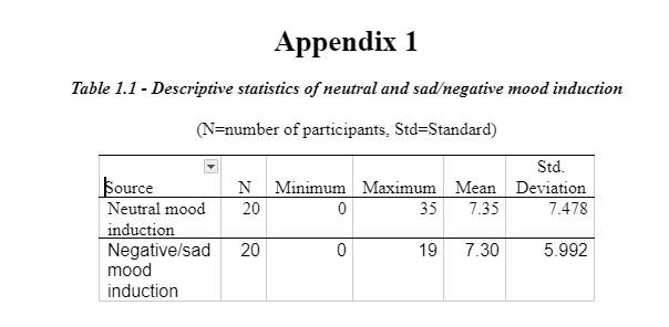
A transformation process of applying an addition mathematical function to all of the ten negative mood scores of the POMS (NervousT + LonelyT + UnworthyT + TenseT + AnxiousT + DiscouragedT + UneasyT + GloomyT + SadT + ShakyT), was conducted to provide a total score of POMS (Profile of Mood States) of the negative mood items for each participant. A new data variable with the name ‘TotalPOMS' was created in the data file. To obtain separate descriptive statistics for each group which was the neutral and negative mood induction group, a split file was conducted to organise the groups. An analysis of the descriptive statistics was then performed to form a trait negative mood score for each group (neutral and negative induction group).

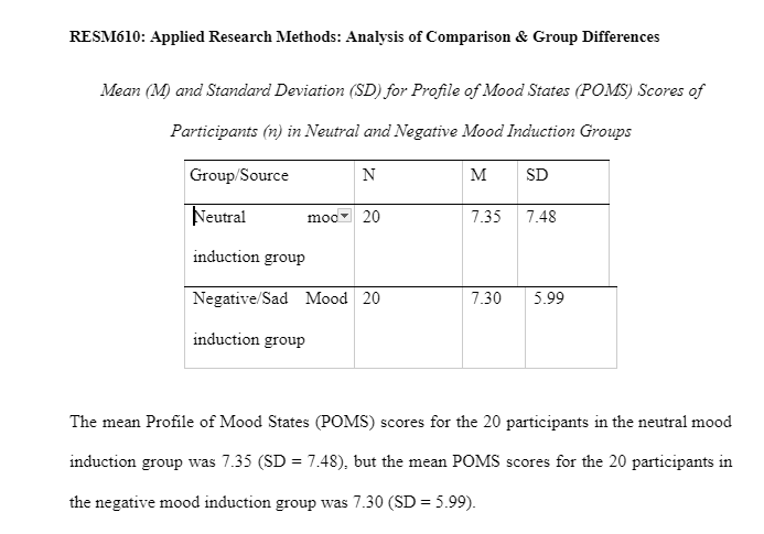
The data in Table1 indicates that the means scores of the two groups for neutral mood induction (7.35) and negative mood induction groups (7.30) for trait negative mood were similar for the 20 participants. The standard deviation shows the amount each group varies from the mean. The group in the neutral mood induction group shows a standard deviation of 7.48 and the negative mood induction group shows a standard deviation of 5.992. The variability in the neutral mood induction group is higher than that of the negative mood induction group. As shown in Appendix 1 – Table 1.1, this could account for the maximum score in the neutral mood induction group being 35 in comparison to the negative mood induction group being 19.

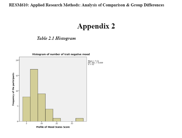
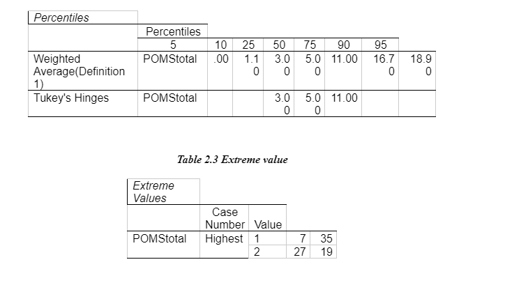
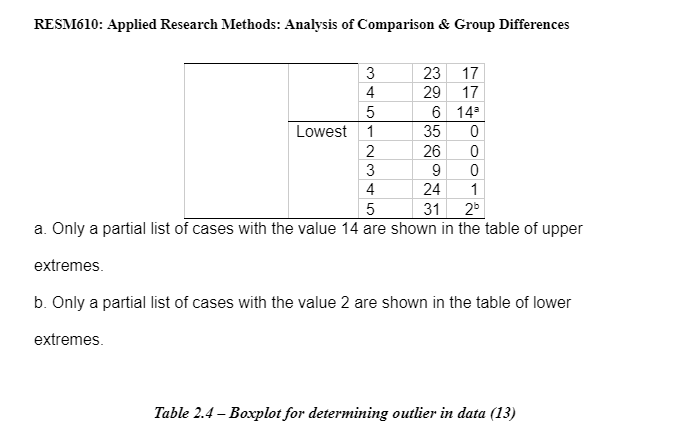
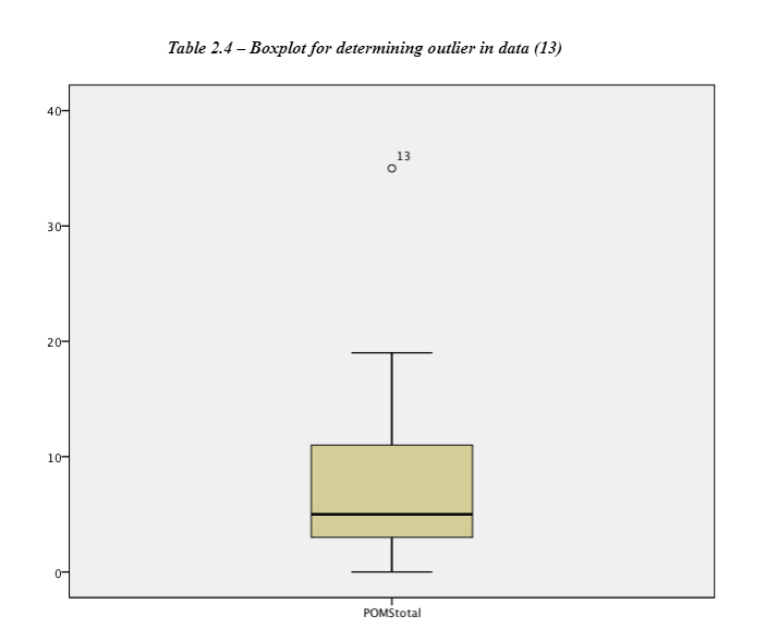
An independent sample t-test was used to assess whether they were significantly different for the dependent variable; the negative mood scores in the standard deviation of the two groups. This will establish whether the two means collected from the independent samples (neutral and negative induction groups) differ significantly (Lesaffre, et al. 2009). As observed above in Table 1 the descriptive statistics have been presented. The sample groups meet the parametric assumptions of equal variance and there being a homogeneity of variance. The data met the t-test assumptions of a t-test in that, (1) scales of measurement being continuous or ordinal scale, (2) it is a random sample from the population, (3) the data is the characteristic that is normally distributed in the population, (4) groups are independent of each other and (5) population variance are equal (André-Obadia et al., 2006). The normal distribution was found by looking at the total of the POMS scores from data output in the form of a histogram to show how the distribution looks and if there a possible outlier in the data set (shown in Appendix 2 – Table 2.1). A boxplot was created to identify which participant was the outlier which was then removed from the data. To make sure the population variance is equal; participant 13 was removed from the dataset for the independent samples t-test (Table 2.4).

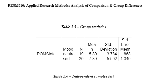
The independent samples t-test results (See Appendix 2 – Table 2.6) show there was not a significant difference in the scores for neutral mood induction group independent variable (N=19, M=5.89, SD=3.78) and the negative/sad mood induction group (N=20, M=7.30, SD=5.10) condition; t=(37)=-0.87, p=0.39. The confidential intervals difference between the two groups 735-7.30=0.05. Levene’s test result show that if p>0.05, we accept the variable. This means that the variance is not significantly different so we can assume that they are equal. These results suggest that the mood induction group do not differ significantly on the trait negative mood.

The two groups rated their level of sadness at three-time points. Use an appropriate ANOVA design to analyse the VAS sadness data and assess whether the mood induction achieved its aim.

Would you have preferred to use MANOVA to analyse the data from the four visual analogue scales? What design could have been used for this analysis? What would have been the advantages or disadvantages of doing this?

A 3 X 2 mixed model ANOVA was conducted to assess if acute negative mood affected attention control on the Visual Analogue Scales (VAS) on the ‘sad' indices. The first condition was the dependent variable which had three levels of time when the VAS sad indices were scored; a before mood induction (BMI), after mood induction (AMI) and after flanker task (AF). This was a repeated measure of the factor within the same participants. In the second condition, there were two independent variables or ‘fixed factor’ variables; the participants were allocated to both a neutral mood induction and a negative mood induction which is a between subjects’ factor.

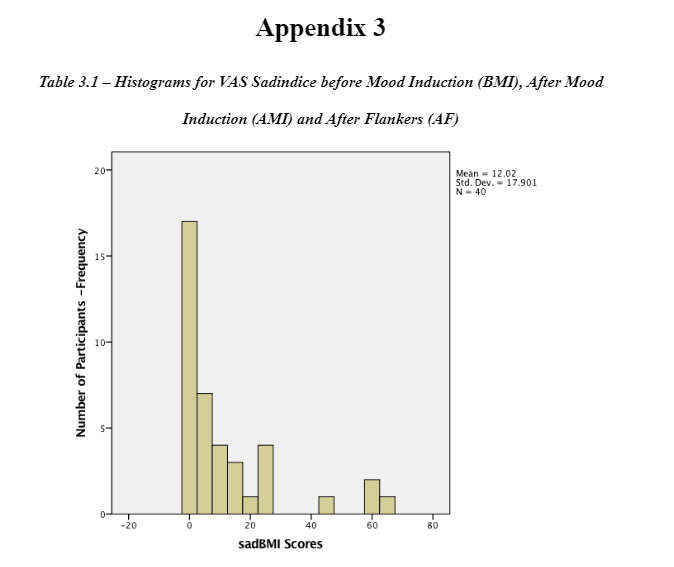
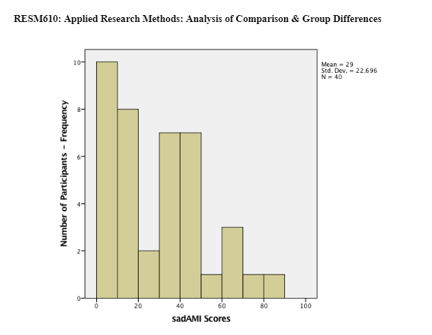
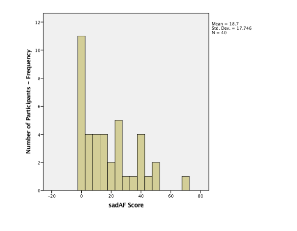
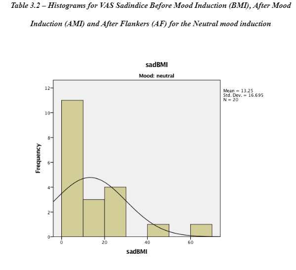
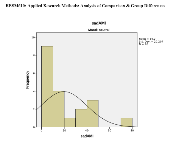
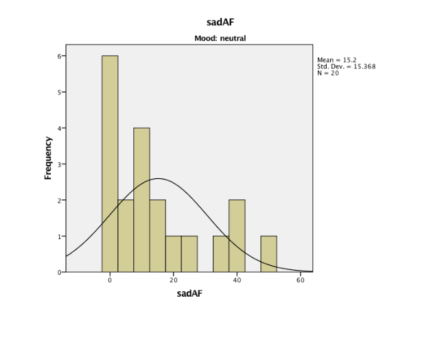
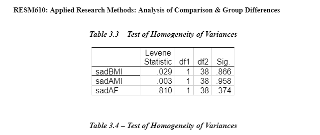
A mixed model ANOVA develops upon the one-way repeated measures ANOVA within subject’s design (Lesaffre, et al., 2009). It accounts for the variation between individual participants and the differences of participants when scoring the VAS sad indices at different time intervals. A repeated measure design has increased power because it removes the individual difference between participants providing a more accurate effect or manipulation of the mood induction in the two groups (Field, 2005). The assumptions for a mixed model ANOVA are that (1) the dependent variable is a measured variable in an interval or ratio data. In this case, it is the time intervals on the level of the sad index. The participants' score on the VAS sad index is a vertical line from ‘Not at all' to ‘Extremely.’ (1) The data is a normal distribution and (3) homogeneity of variance. This data, shown in Appendix 3 – Table 3.1 and 3.2 shows a positive skewness in the VAS sad index. Notably, a transformation could be completed but since there is no a bootstrapping option for the mixed model ANOVA, it could not be completed. The VAS sad scores have a normal distribution. The Levene's static was conducted using a one-way ANOVA for the homogeneity of variance of the three levels of the VAS sad index. There is the homogeneity of variances across the three levels as shown in Appendix 3 – Table 3.3.

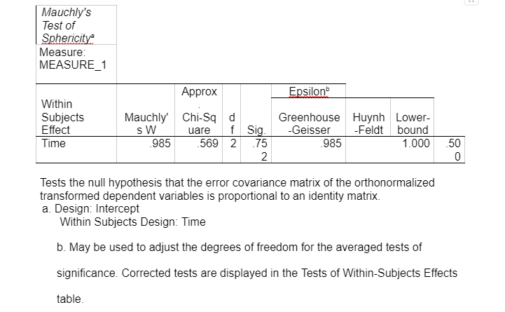
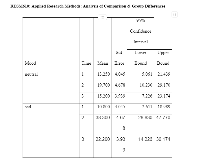
Sphericity is a crucial assumption of a repeated-measures ANOVA and mixed model ANOVA. It refers to the condition where the variances of the differences between all possible participants of within-subject conditions, for example, the neutral and negative mood induction groups are equal (Statistics-help-for-students.com, 2017). The Mauchly's test of sphericity for repeated measures indicates the main effect of time does not significantly violate the sphericity assumption because the significant value is greater than 0.05, x2(2) = 0.077, p=0.962. Resultantly, the F-value for the main effect of time (and its interaction between the mood inductions variable) does not need to be corrected for the violation of sphericity. The means and standard deviation of the standardised score on the VAS sad indicate, the three-time intervals for each mood induction are presented and some participants in each group in Table 2.

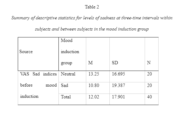
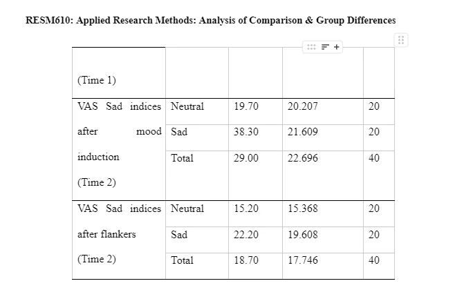
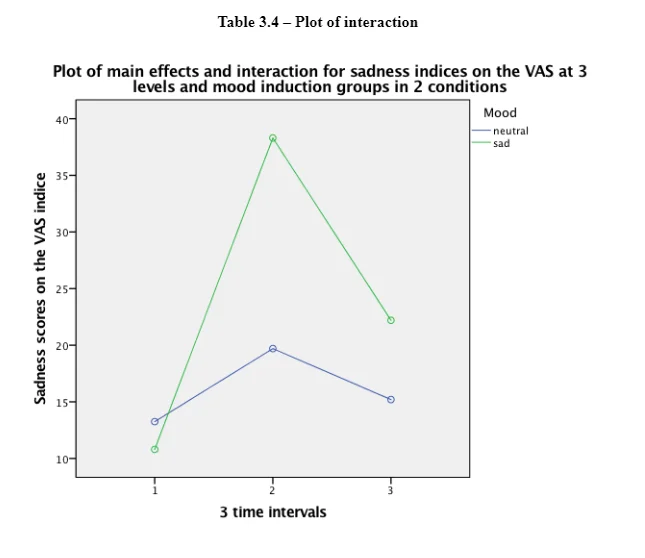
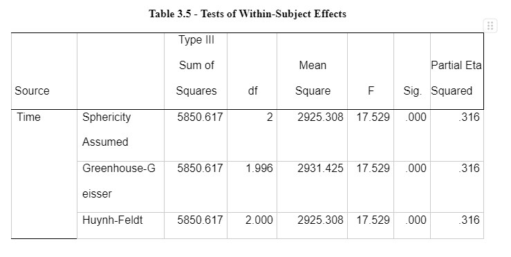
This data on the means indicates that the sadness index level increased at time 2 (after mood induction) and decreased at time 3 (after flanker task). The sad/negative mood induction group shows high levels of sadness in comparison to the means on the neutral mood induction group. The standard deviations remain consistent within and between subjects. Interaction has been shown in Appendix 3 – Table 3.4. It shows an exponential interaction where the lines are in the same direction, but one is steeper than the other. Table 3.5 shows there is a significant interaction between time intervals on sadness scores and the mood induction. There was a main effect at the time intervals (before mood induction, after mood induction, after flanker task), F(2, 76) = 2925.308, p = 0.00, np2 = .316. The main effects of time at the three intervals (before the mood induction, after the mood induction, and after the flanker's tasks) changed their sadness scores on the VAS in the different time intervals (Lesaffre, et al., 2009). The time intervals x mood induction interaction was significant F (2, 76) = 6.661, p = 0.02, np2 = .149. This shows different sadness scores on the VAS over time, and it was different in the different conditions; participants were put into either neutral mood induction group or the negative/sad induction group.

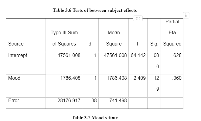
The main effect of the condition of mood induction groups (neutral and negative/sad) was not significant F (1, 38) = 0.2.409, p= 0.129, np2 = 0.06. There was no significant difference in mean VAS sadness scores between the groups shown in Table 3.6. Table 3.7 provides a breakdown of the time intervals (before mood induction, after mood induction, after flankers task). The sadness scores on the VAS after the mood induction were the highest after the negative/sad mood induction (M=38.3). The scores before the mood induction in the group in the negative mood induction were lower (M=10.8) than those who were given the neutral mood induction (M=13.250). This suggests that the score of the negative induction group remained high after the mood induction (M=38.3) and the flanker's task (22.2) compare to the neutral induction mood group. The results of the 3 x 2 Mixed ANOVA show that the mood induction did significantly change the VAS sadness scores for the two groups and there is no a significant different between the two groups for the mood induction. MANOVA would have been preferred to be used to analyse the data from the four visual analogue scales. A mixed model ANOVA which compares two or more categories independent variable (>2 groups) on one continuous dependent variable was completed for the sadness VAS scores. This could be further developed with more than one continuous dependent variable using MANOVA. As there are 4 VAS levels, this would create more than one continuous dependent variable (sad, happy, anxious, bored) with a further three levels in the time interval the scores would be collected (before mood induction, after mood induction, and after flankers task).

Applied Research Methods: Analysis of Comparison & Group Differences

A repeated measure MANOVA could be completed for this analysis since there are several dependent variables in two experimental conditions (Enders, 2003). For this case, the variables would be sad, happy, anxious and bored as at before mood induction, after mood induction, and after flanker’s task. It would be a 4 x 3 x 2 mixed model MANOVA design. This is because the independent variable of the groups is between-subjects factors with four levels, while the measurement time-points are repeated measures factors with three levels.

MANOVA would consider correlations between dependent variables and be able to identify the differences. MANOVA is a different way of looking at the mixed model or repeated measures design. It uses the material on multivariate tests generated in mixed model ANOVA. It considers the same assumptions of the ANOVA in the data being interval/ratios, normally distributed, observations independent and random samples. As this is a sample size of 40, an MANOVA does not consider sphericity due to it error terms. It makes the variance stable and reliable. If the sample sizes were unequal, MANOVA in SPSS offers adjustment of the unequal sample sizes. It assumes homogeneity of variance and covariance. The dependent variable show equal levels of variation across the range of levels. (sad, happy, anxious and bored and the three-time intervals). It also considers a multivariate design with multiple dependent measures. MANOVA allows for a different dependent variable within-subject independent variable with many levels.

Limitations of an MANOVA, in this case, is the sensitivity to outliers, and the difficult to identify which type of error is occurring in an analysis. The problems with running a multiple ANOVA would be the increase in familywise error rate. The problem with MANOVA could be if the dependent variable is not empirically linked to be correlated making it difficult for MANOVA to have any value.

Flanker task

For the flanker task part of the study, there were three factors in the design (mood (1), congruence (2), and spacing (3)). Use an appropriate ANOVA design to analyse this data and consider whether the mood induction affected distractibility by incongruent distractor stimuli, and how this was affected by the spacing of stimuli?

Would it be helpful to use either: i, errors made in the flanker task; or ii, reaction time for trials with no noise stimuli, as a covariate in the analysis of the flanker task data?

A 3 x 2 MANOVA design will be used to analyse this data and consider whether the mood induction affected distractibility by incongruent distractor stimuli. The dependent variables include incongruent variable (SpacingNarrowingIncongruent, SpacingIntermidateIncongruent and SpacingWideIncongruent) where the noise letter are different from the target and their reaction times (Nieuwenhuis, et al., 2006). The independent variables are the mood induction groups (neutral and negative/sad) and if they influenced reaction times (RTs) on the incongruent targets.

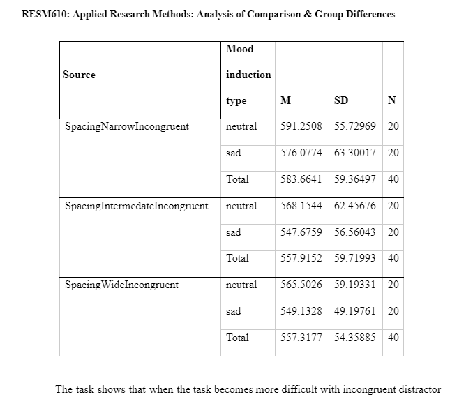
The task shows that when the task becomes more difficult with incongruent distractor stimuli of the noise letters different from the target shows, reaction time slows overall on the narrow spacing of letters and similar reaction times for the intermediate and wide spacing of letters.

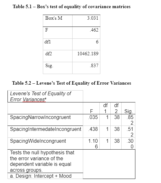
The assumption is the homogeneity of covariance matrices: Box’s test is non-significant (Enders, 2003). These indicated covariance matrices are equal enough, see Appendix 5 – Table 5.1.

The Levene’s test is non-significant (See Appendix). Therefore, there are equal variances amongst groups for each incongruent dependent variable (SpacingNarrowingIncongruent, SpacingIntermidateIncongruent and SpacingWideIncongruent).

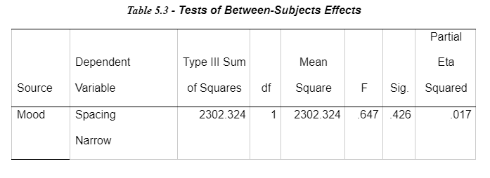
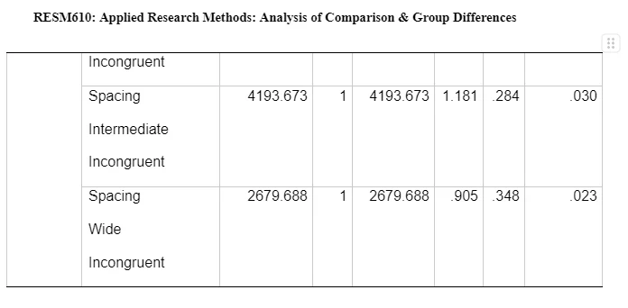
A one-way ANOVA for each dependent variable has been completed shown in Table 11. The separate univariate ANOVAs on the outcome variable for timings on the Flanker task revealed non-significant effects on the mood induction groups and on incongruent noise letters on narrow spacing, F(1,38) = 0.647, p>.05, on incongruent noise letters on intermediate, F(1,38) = 1.181, p>.05 and on incongruent noise letters wide, F(1,38) = 0.905, p>.05. See Table 5.3 for more details.

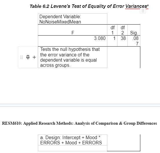
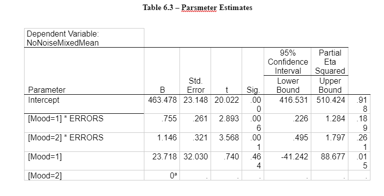
An ANCOVA needs to be completed to reduce the size of the error variance within groups and therefore increase the sensitivity of the between group comparison on the mood induction. A covariate in an ANOVA is also completed to minimize confounding variables, for example, the errors on the Flankers tasks on participants’ reaction time on the Flankers task (Statistics.laerd.com, 2017). A decision needs to be made about a variable that could influence the dependent variable as a covariate but not to the two allocated groups to the different mood inductions. Therefore, a check needs to be made to determine if the errors made on the flanker's task ‘ERRORS’ influence the reaction time with no noise influence the dependent variable ‘NoNoiseMixedMean.’

The assumptions are the same as an ANOVA (normal distribution, interval data, and independent scores) but also include additional points for consideration of the (1) groups should not differ on the covariate(2) independence of the covariate no noise reaction times effect and errors made on the flankers task (covariate must have a linear relationship to the dependent variable) and (3) homogeneity of regression slopes, the regression lines for the separate groups should be parallel (Krabbe and Weijnen, 2003).

Two independent t-tests was conducted using the two mood induction groups as independent variable the covariates as the outcomes ‘ERROR’ and ‘NoNoisedMixedMean.’For no noise mixed mean there was not a significant difference between the scores for neutral mood induction(M=544.43.08, SD=56.69135) and sad/negative mood induction (M=538.0788) conditions; t(38)=0.369, p=0.714. For error on Flankers task, there was not significantly different between the scores for neutral mood induction (M=75.85, SD=39.05095) and sad/negative mood induction (M=65.1000, SD=31.71402) conditions; t(38)=0.956, p-0.345, see Appendix for output. As there is no significant different, we can proceed with the ANCOVA.

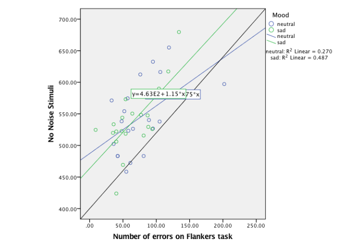
A correlation between reaction time with no noise stimuli and number of errors on the flanker's task. This was to determine if there were no relationship there would be no adjustment. There was a low significant correlation (0.596), and an ANCOVA can be proceeded with.

The test for the assumption of homogeneity of regression slopes explores the relationship between the covariate number of errors on Flankers task and the dependent variable for reaction times with no noise stimuli need to be the same for each of the moods (Verbruggen, et al., 2006). A correlation was completed, and a regression line was used to show if there was a relationship shown in Appendix 6- Table 6.1. An interaction between the no noise stimuli and the number of errors on the flanker's task was no significance; therefore, the lines were parallel enough. Therefore, it met the assumption of homogeneity of regression slopes.

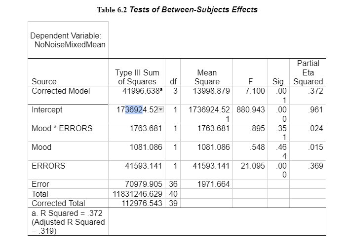
An ANCOVA found that after controlling errors made on flanker task, there was still a significant effect of mood induction groups on no noise reaction time F(1,37) = 0.01, np2= 0.02. See the output in Appendix 6 – Table – 6.2 to 6.3.

References

• André-Obadia, N., Peyron, R., Mertens, P., Mauguière, F., Laurent, B., & Garcia-Larrea, L. (2006). Transcranial magnetic stimulation for pain control. Double-blind study of different frequencies against placebo, and correlation with motor cortex stimulation efficacy. Clinical Neurophysiology, 117(7), 1536-1544.
• Enders, C. K. (2003). Performing multivariate group comparisons following a statistically significant MANOVA. (Methods, Plainly Speaking). Measurement and Evaluation in Counseling and Development, 36(1), 40-57.
• Field, A.P. (2005). Discovering Statistics Using SPSS (second edition). London SAGE
• Krabbe, P., & Weijnen, T. (2003). Guidelines for analysing and reporting EQ-5D outcomes. In The measurement and valuation of health status using EQ-5D: A European perspective (pp. 7-19). Springer Netherlands.
• Lesaffre, E., Philstrom, B., Needleman, I., & Worthington, H. (2009). The design and analysis of split‐mouth studies: What statisticians and clinicians should know? Statistics in Medicine, 28(28), 3470-3482.
• Nieuwenhuis, S., Stins, J. F., Posthuma, D., Polderman, T. J., Boomsma, D. I., & de Geus, E. J. (2006). Accounting for sequential trial effects in the flanker task: Conflict adaptation or associative priming? Memory & Cognition, 34(6), 1260-1272.
• Statistics-help-for-students.com. (2017). Statistics Help for Students. [Online] Available at
• Statistics.laerd.com. (2017). Features - Writing Up | Laerd Statistics. [Online] Available at:
• Statistics.laerd.com. (2017). Features - Writing Up | Laerd Statistics. [Online] Available at:
• Verbruggen, F., Notebaert, W., Liefooghe, B., & Vandierendonck, A. (2006). Stimulus-and response-conflict-induced cognitive control in the flanker task. Psychonomic Bulletin & Review, 13(2), 328-333.

Dig deeper into Diet and iron status with our selection of articles.