Dispersion and Market Risk Measurement

INTRODUCTION

Dispersion as a statistical term defines the range of values that are expected for a particular variable (Christie, William, and Huang, 1995). A good example is the familiar risk measurement, Beta, which measures the dispersion of a security`s returns relative to a particular market index or benchmark. In the event that the dispersion is greater than that of the benchmark, the security is perceived to be riskier when compared to the benchmark (Christie, William, and Huang, 1995; Chang, Cheng, and Khorana, 2000). On the other hand, if the dispersion is less, then it is perceived not to be as risky as the benchmark. A beta measure of 1.0 would be an implication that an investment is moving in unison with the benchmark. A beta of less than 0 implies movement that is contrary to the benchmark, while a beta of 0 signifies no correlation. For example, if using the S&P as a benchmark, an investment portfolio has a beta of 1.0, the movement between the benchmark and the portfolio is almost identical. On a negative beta, the portfolio moves in the exact opposite direction if the S&P 500 is up, which will move down in this case. Correlation is another term that a considerable number of researchers have used, in place of dispersion, in conducting their analyses in trying to understand the behaviour of stock prices and returns (Pollet and Wilson, 2010). However, although related, correlation is different from dispersion; it is the obverse of it, where it rises as dispersion falls, and also is a pure number below 1, and not a rate (Driessen, Maenhout, and Vilkov, 2009).

At this point, thus, it is important to note that market participants investment behaviour has been linked to different factors like investor`s investment horizon which is the benchmark used for measurement of performance, other market participants behaviour, underlying markets volatility degree, and the presence of speculative trading activity and fads in the financial markets. The above is the one of the main focus areas that past researchers have dwelled on, and thus, this dissertation takes a different turn. In this dissertation, the researcher is going to test whether both dispersion and correlation behave differently in good times and bad. Thus, the research question is stated as follows:

Research Question: Do both dispersion and correlation behave differently in good times and bad?

LITERATURE REVIEW

Factual Information Regarding the Topic

As introduced earlier, dispersion refers to the difference between the worst and the best performers in an index or a collection of securities (Beaver, 1970), while correlation is a measure of any two variables like two stocks that match one another with regards to their performance in a given period (Sharpe and William, 1991). According to Sharpe and William (1991), a portfolio manager who controls a fortune needs diversification. A valid claim regarding the index’s internal diversification and its overtime variation requires quantitative metrics. In this regard, therefore, the commonly encountered statistics is that of correlation, but is still with its flaws. Thus, a measure of asset dispersion has proven to have strong qualifications to be a complementary tool (Sharpe and William 1991).

Analysis of the Relevant Issues around the Topic

Equity Portfolios

Being in a “stock-picker’s market” is a phrase used which is used often. Philips (2012) argues that dispersion, as opposed to correlation, provides a way of measuring the stock’s potential value needed for selection ability. During good economic times, active investors always find it challenging in conducting a beating index portfolio. In such scenarios, a passive investing case unusually requires urgent attention (Bechmann et al., 2013).

Vitality

Philips (2012) further suggests that a higher dispersion can comprise of both the bear and bull markets. The claim is counter-intuitive regarding the negative correlation between the market performance and vitality; a high dispersion might be expected for high vitality (Bekaert and Harvey, 2000).

Factor Importance

At the best description of risks, it is necessary to consider the specific factor exposures. For instance, the challenge of the suitability of international equity as calibrated by a sector has received much attention (Chang et al., 2000). Furthermore, Philips (2012) illustrates that the essential multi-asset diversification’s metric only captures a section of historical returns. Dispersion provides the best complementary input that quantifies idiosyncrasy extent in component performance (Chiang et al., 2000). Correlation, on the other hand, suffers from critical challenges during economic times including being fooled by the complexity, in that it shows a relationship of a perfectly straight line. Thus, a zero correlation does not indicate independence, and, therefore, correlation cannot capture a relationship in a straight line (Boreinstein and Rose, 1994; Cheng and Warfield, 2005; Shneider, 2003; Tim and Craig, 2013).

Assessing Different Interpretations and Arguments (of Whether or Not Dispersion and Correlation Behave Differently during Good and Bad Times)

Henderson (2017) argues that during good and bad economic times, correlation can be crucial in aiding the investors and fund managers to diversify. For instance, the consideration of the behavior of two financial stocks at the announcement of the interest rate and their difference in performance can be adequately addressed by correlation. Similarly, Czanitzki and Kraft (2009) report that it is possible for the investors to use correlation while exploring the relationship that exists between various asset classes. Consequently, during bad economic times, the managers can produce performance levels versus the average of the index (Plazzi et al., 2008). The authors insinuate that at good economic times, the fund managers have more chances of generating the additional returns through the process of identifying the winners. According to Chiang and Jeon (2007), stock dispersion is particularly important while assessing outperformance potential of the particular index over a given period. It is worth considering certain fund managers who have the stock-picking ability at the times when stock markets exhibit improved dispersion levels (De Bondt and Thaler, 1985; Henderson (2017).

With regards to the context of correlation, the researchers have indicated that many related commentaries for increasing the stock correlation during economic times have mainly focused on the current time frames. However, long-time analysis of correlation gives a broader perspective. The same scholars continued to provide evidence that even though correlation can change within a particular period, the recent drops and spikes in correlation are not unprecedented (Evans and Archer, 1968; Freeman, 1988; Nelson and Plosser, 1982). The higher magnitude indicates greater dispersion while on the other hand, the less magnitude shows less dispersion, and thus, regardless of the correlation and dispersion of returns, in aggregate almost half of the dollars that are invested in index securities will underperform and half outperform (Gilmore, et al., 2008; Malkiel and Fama, 1970; Racheve, et al., 2010). According to Longin and Solnik (2001), dispersion opportunities persist through the market change. They argue that observing the recent years indicates the mentioned opportunities. As per their findings, they said that the first years provides bear, a bull as well as flat markets, however, the dispersion’s degree is always reasonably the same (Henderson, 2017; Jegadesh and Titman, 1993; Shiller, 2003).

Summaries of the Literature and Research Gaps

It is evidence, from the literature, that there are only few authors that have discussed how dispersion and correlation behave differently during good and bad economic times. Most of the articles were mainly focused on the relationship and the comparison between correlation and dispersion. Generally, there is more to be done to (regarding the literature) determine different behaviours between correlation and dispersion during good and bad economic times.

DATA AND METHODOLOGY

The paper focused on determining whether both dispersion and correlation behave differently during good times and bad. There is the need to, therefore, understand the behaviour under consideration, which in this case implies the change in the movement of the dispersion and correlation values and their magnitudes. The meaning of behaviour in this case is taken to mean the increase or decrease of dispersion and correlation values, where it is tested whether both change in a similar way, and in almost equal magnitudes.

Given the above, it was important to obtain market data on asset portfolios where this data would be used to calculate dispersion as well as correlation. For the case explained in the previous statement, data was extracted from Yahoo Finance. From Yahoo Finance, real time data on stock prices, dividends, and beta (representing risk) were obtained and exported to excel for analysis. Here, the new formula for calculating dispersion was used from which the dispersion values were further used in the calculation of correlation. The equations are as presented below:

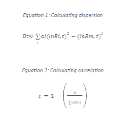
Where;

Dt = Dispersion in period t

ai = Weight of asset in the market portfolio (non-negative and sum to 1)

Ri,t = Total excess return on a security i, and in period t

Rm,t = Market return in period t

Rvi = Variance of the index

c = Correlation

Using the formulas above, dispersion and correlation were calculated from a data set of daily historical stock prices and dividends, from 24th August 2017 to 24th August 2018. Since it was daily data, a period of one year was enough to produce the many data points required to produce useful trends for comparisons of the behaviours of dispersion and correlation at different times.

It is also important to note that good and bad terms were decided, in the simplest terms of all, to be where the market returns are positive and negative respectively, and not necessarily increasing or decreasing. Therefore, during analysis, the movement of dispersion as well as correlation values would be checked, to determine whether or not they move in similar directions and magnitudes. This is the basis of comparisons that was set for use in this report. The rationale behind the basis of comparison as explained before and above, is that it allows the researcher to compare the trends of both dispersion and correlation over a long period. These trends can be done collectively, where both good and bad times are grouped together, or separately for the good and bad times. All of these approaches offer a clear and direct way of understanding the behaviour of both dispersion and correlation in good times and bad.

DATA ANALYSIS

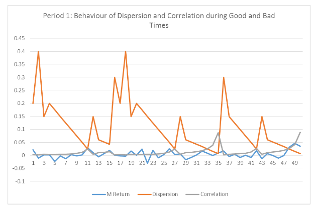
Figure 1 above indicates that from data point 1 to 11, dispersion sharply rises and falls at the same time, while correlation is constant for the larger part, and towards point 11 rises. This is repeated between points 11 and 27, 27 and 35, and 35 and 42 as well as 42 and 49. Between the identified points above, the market experiences both good and bad times and while the market return increases, dispersion falls while correlation increases. That is, the figure shows high correlations during high and positive market returns while at the same time shows low dispersion.

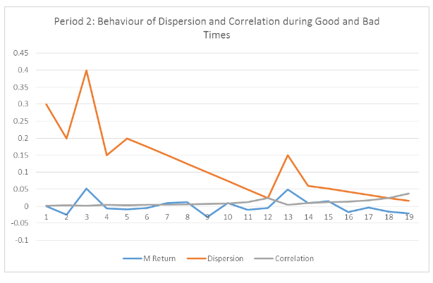
Figure 2 presents a significantly different scenario particularly on the movement of dispersion values versus those of market return. As it is seen from point 1 to 8, the dispersion fall as market return fall and rise as market return grows towards the positive. As regards correlation, it takes the behaviour of dispersion as depicted in Figure 1, where market returns fall as it rises. Despite the above, the behaviour under consideration is rarely seen as correlation remains constant for longer periods than it changes. Particularly, from point 1 to 10, market returns show both negative and positive values in alternate, but correlation remain unchanged, which is not the case with dispersion.

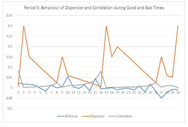
Figure 3, in the third excerpt above, depicts an almost similar behaviour as that witnessed in figure 1. In point 1, 8, 16, and 26, the troughs and peaks of both dispersion and correlation collide indicate a significant difference in behaviour, during any economic time, whether bad or good. Furthermore, this period presents complex and confusing results in which at some point both dispersion and correlation move in similar direct as the market return. What is clear, even from the previous periods, is that the magnitude of change for the dispersion is much higher as compared to that of correlation, even though there are no significant differences of market returns during both good and bad times. In addition to the above, the fact that troughs and peaks of both and dispersion mostly collide, the implication is that these two behave differently during different times. Up to this point, what cannot be answered with facts (in specific terms) is whether one increases or decreases or behaves the other way round, as the market changes from good to bad times or vice-versa.

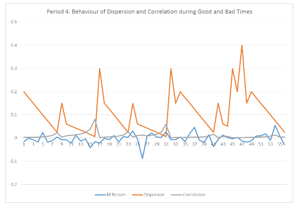
Figure 4 depicts a similar situation as in figures 1 and 3. Dispersion fluctuates with high peaks and deep troughs indicating a cyclic behaviour and mostly this goes in the opposite direction as correlation. As in the previous four periods, correlation is mainly constant and rarely changes as the market moves from good to bad times. Despite the above, where the market returns fall, correlation increases indicating (note that correlation is positive throughout) and does it does not change direction to the negative but only moves slightly, positively. Here, it is clear that correlation is moving in a different direction and with different magnitude as compared to dispersion. This is evident in point 9, 16, 23, 31, and 41.

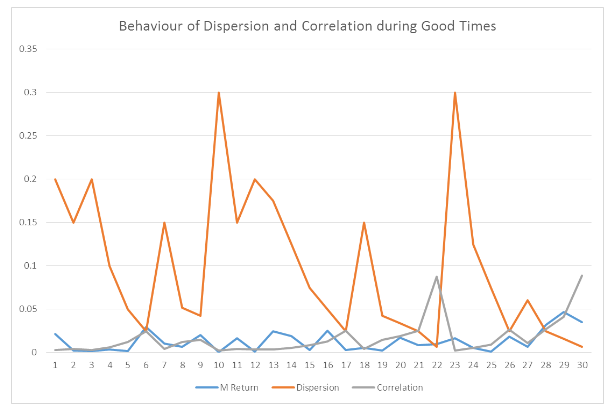
Figure 5 above indicates that dispersion is high when correlation is low. As seen at point 1, 6, 17, 26, 27, and 28, dispersion and correlation move in the opposite direction.

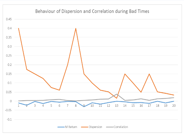
Figure 6 above shows a slightly different scenario from that seen in figure 5, where correlation in most of the times is constant. It is only at one point that it rises while dispersion falls. As regards dispersion, it behaves in a similar manner as depicted in figure 5.

EVALUATION AND INTERPRETATION OF FINDINGS

From the literature review, it is clear that the topic of whether both dispersion and correlation behave differently during bad and good times is not widely explored. Thus, there are few arguments regarding how dispersion and correlation behave during different times. As stated before, good and bad times is taken to mean when the returns are positive and negative respectively. Thus, the behaviour of the two is only analysed and compared based on the above, although it should not be ignored that good times can mean the period when returns rise significantly, even if it means only in the positive or negative side. This alone shows how complicated, no matter how simple one can view it, comparing the behaviour of correlation and dispersion is. The sentiments above are supported by the data analysis, where, various interpretations can be made, but cannot hold for long. For example, in period 1, 3, and 4 it is obviously clear that dispersion and correlation, collectively, behave differently in good and bad times. This is not the case with period 2, and which bring about some differences as regards the direction and magnitude of change of dispersion and correlation in both bad and good times. The implication here is that out of four periods of analysis, the difference between dispersion and correlation’s behaviour in good and bad times is only seen thrice. This further implies that as time moves to the long-run, the comparison gets more complicated, with varying results.

The other point to consider is what the basis of comparison is; dispersion in good times vs. dispersion in bad times, correlation in good times vs. correlation in bad times, or correlation and dispersion in bad times vs. good? With the latter, based on the data analysis, it is evident that in most cases the difference is present while for the two former, there is no significant difference. That is, dispersion would behave differently between good and bad times, from correlation, and not itself. This is the same case with correlation, which even shows the difference throughout the four periods used. Going back to the argument of the comparison being complex, how dispersion behaves (in terms of direction and magnitude of change) is almost similar in all cases but not the same, which is a similar case, but not equally the same with correlation. Thus, on one hand, how dispersion and correlation (not in comparison with the other) behave during both bad and good times cannot be said, in specific terms, to be similar or different. On the other hand, how dispersion and correlation (in comparison with the other) behave during both bad and good times is completely different. That is, their movements in terms of direction and magnitude are opposite of one another (Pollet and Wilson, 2010; Driessen, Maenhout, and Vilkov, 2009; Christie, William, and Huang, 1995; Chang, Cheng, and Khorana, 2000).

Further complexity is identified when the good times and bad times are completely separated from one another, as seen in Figure 5 and 6 respectively. Dispersion is shown to be high when correlation is low (dispersion and correlation move in the opposite direction with different magnitudes), during good times just as in established in the previous analysis. On the contrary, where more complication is experienced in bad times, as there is a slight difference, where correlation in most cases is constant. It changes only at one point while dispersion behaves in a similar manner as depicted in good times. The analysis here further cements the general conclusion that the behaviour of dispersion and correlation is different in both good and bad times (Christie, William, and Huang, 1995; Chang, Cheng, and Khorana, 2000). This conforms to the fact that, as supported by literature, high correlation depicts low dispersion, and this is the same in both cases of bad times and good (Pollet and Wilson, 2010; Driessen, Maenhout, and Vilkov, 2009; Christie, William, and Huang, 1995; Chang, Cheng, and Khorana, 2000).

CONCLUSIONS

This dissertation aimed at testing whether both dispersion and correlation behave differently during good times and bad. A series of procedures were undertaken to complete the test, where market data from Yahoo Finance was used to facilitate the reaching of this dissertation’s aim and objective. The new formula for measuring dispersion was used, and the said dispersion obtained was used to find out what its corresponding correlation was. This was done after a considerable consideration of the existing literature on the topic, which was very limited. The limited literature is a firm evidence that the research question under consideration is yet to be explored from different perspectives of different researchers. Thus, it was necessary to conduct the test as introduced earlier. Despite the limitations encountered as regards the literature on the topic, what was important was the development of a procedure which could provide the correct results in measuring both dispersion and correlation. Here, the new formula for dispersion was used, but the results obtained as well as their analysis do not present firm evidence that the formula is useful in terms of understanding the movement of asset returns, and thus it can be termed as a tentative way of understanding the behaviour differences under consideration. Consequently, it cannot be clearly said that it was the most useful way of understanding the behaviour of dispersion and correlation during both bad and good times. As established in the results analysis and evaluation and interpretation sections, it is very clear that both correlation and dispersion behave differently during bad and good times (this explains the difference in behaviour between correlation and dispersion). However, given that some periods of analysis depicted some differences from others, the evidence is questionable and tentative, and thus should be subjected to further testing. This can be achieved through the use of different formulas of measuring dispersion, or conducting a replica analysis as in this dissertation, but comparing different markets (assets in different markets). With regards to independent behaviour of each one of the two (dispersion and correlation considered independently-compared to itself in bad and good times), the behaviour is similar, and this is where the evidence is firm.

REFERENCES

Bachmann, R., Elstner, S. and Sims, E.R., 2013, “Uncertainty and economic activity: Evidence from business survey data” American Economic Journal: Macroeconomics, 5(2), pp.217-49.

Beaver, W.H., 1970, “The time series behavior of earnings” Journal of Accounting Research, pp.62-99.

Bekaert, G. and Harvey, C.R., 2000, “Foreign speculators and emerging equity markets” The Journal of Finance, 55(2), pp.565-613.

Borenstein, S. and Rose, N.L., 1994, “Competition and price dispersion in the US airline industry” Journal of Political Economy, 102(4), pp.653-683.

Chang, E.C., Cheng, J.W. and Khorana, A., 2000, “An examination of herd behaviour in equity markets: An international perspective,” Journal of Banking & Finance, 24(10), pp.1651-1679.

Chang, E.C., Cheng, J.W. and Khorana, A., 2000, “An examination of herd behavior in equity markets: An international perspective” Journal of Banking & Finance, 24(10), pp.1651-1679.

Cheng, Q. and Warfield, T.D., 2005, “Equity incentives and earnings management” The accounting review, 80(2), pp.441-476.

Chiang, T.C. and Zheng, D., 2010, “An empirical analysis of herd behavior in global stock markets” Journal of Banking & Finance, 34(8), pp.1911-1921.

Chiang, T.C., Jeon, B.N. and Li, H., 2007, “Dynamic correlation analysis of financial contagion: Evidence from Asian markets” Journal of International Money and finance, 26(7), pp.1206-1228.

Christie, William G., and Roger D. Huang, 1995, "Following the pied piper: Do individual returns herd around the market?" Financial Analysts Journal, 51(4), pp.31-37.

Connolly, R. and Stivers, C., 2003, “Momentum and reversals in equity‐index returns during periods of abnormal turnover and return dispersion” The Journal of Finance, 58(4), pp.1521-1556.

Czarnitzki, D. and Kraft, K., 2009, “Capital control, debt financing and innovative activity” Journal of Economic Behavior & Organization, 71(2), pp.372-383.

De Bondt, W.F. and Thaler, R., 1985, “Does the stock market overreact?” The Journal of finance, 40(3), pp.793-805.

Demirer, R. and Kutan, A.M., 2006, “Does herding behavior exist in Chinese stock markets?” Journal of international Financial markets, institutions and money, 16(2), pp.123-142.

Diether, K.B., Malloy, C.J. and Scherbina, A., 2002, “Differences of opinion and the cross section of stock returns” The Journal of Finance, 57(5), pp.2113-2141.

Döpke, J. and Pierdzioch, C., 2000. Stock market dispersion, sectorial shocks, and the German business cycle (No. 966) “Kiel Working Paper”

Driessen, J., Maenhout, P., and Vilkov, G, 2009, “The Price of Correlation Risk: Evidence from Equity Options,” Journal of Finance, 54(3), pp 1377-1406.

Evans, J.L. and Archer, S.H., 1968, “Diversification and the reduction of dispersion: an empirical analysis” The Journal of Finance, 23(5), pp.761-767.

Freeman, R.B., 1988, “Labour market institutions and economic performance” Economic policy, 3(6), pp.63-80.

Gilmore, C.G., Lucey, B.M. and Boscia, M., 2008, “An ever-closer union? Examining the evolution of linkages of European equity markets via minimum spanning trees” Physica A: Statistical Mechanics and its Applications, 387(25), pp.6319-6329.

Henderson Global investors. 2017, “A simple Guide to Dispersion and correlation” … [accessed: 24th august, 2018]

Jegadesh, N. and Titman, S., 1993, “Returns to buying winners and selling losers: Implications for stock market efficiency” The Journal of finance, 48(1), pp.65-91.

Longin, F. and Solnik, B., 2001, “Extreme correlation of international equity markets” The journal of finance, 56(2), pp.649-676.

Malkiel, B.G. and Fama, E.F., 1970, “Efficient capital markets: A review of theory and empirical work” The journal of Finance, 25(2), pp.383-417.

Nelson, C.R. and Plosser, C.R., 1982, “Trends and random walks in macroeconomic time series: some evidence and implications” Journal of monetary economics, 10(2), pp.139-162.

Philips, Christopher B., David J. Walker, and Francis M. Kinniry Jr., 2012, “Dynamic Correlations: The Implications for Portfolio Construction. Valley Forge, Pa.: The Vanguard Group”

Plazzi, A., Torous, W. and Valkanov, R., 2008, “The cross‐sectional dispersion of commercial real estate returns and rent growth: Time variation and economic fluctuations” Real Estate Economics, 36(3), pp.403-439.

Pollet, J.M. and Wilson, M., 2010, “Average correlation and stock market returns,” Journal of Financial Economics, 96(3), pp.364-380.

Rachev, S.T., Hoechstoetter, M., Fabozzi, F.J. and Focardi, S.M., 2010, Probability and statistics for finance (Vol. 176). John Wiley & Sons.

Schneider, J., 2013. European business cycle convergence: portfolio similarity and a declining home bias of private investors “Frankfurt aM: Peter Lang GmbH, Internationaler Verlag der Wissenschaften”

Schulze, W.S., Lubatkin, M.H. and Dino, R.N., 2003, “Exploring the agency consequences of ownership dispersion among the directors of private family firms” Academy of management journal, 46(2), pp.179-194.s

Sharpe, William F., 1991 “The Arithmetic of Active Management. Financial Analysts Journal 47 (1, January/February): 7–9.”

Shiller, R.J., 2003, “From efficient markets theory to behavioral finance” Journal of economic perspectives, 17(1), pp.83-104.