Defect Forecasting

Brief Introduction

This report is as a result of a project-task of conducting some predictive analytics across three aspects of Wattgen, by the company’s operations department. Wattgen worries are that defective parts received from suppliers are too high, there is a high rate of turnover in the company's field service staff, and there is the need for sales and production costs forecasting for effective planning. Given the above, the objectives of this report are to forecast the defects for each of the 18 months based on the data provided, to assess the issues raised by the HR using multiple regression analyses, and forecasting agricultural and industry sales and unit production costs through time series and simple regression analyses. For those seeking guidance in navigating complex analyses, data analysis dissertation help can be invaluable.

Research Strategy
Project stage 1

In this stage, the research considered various techniques including the scatter overlay (scatter plot for multiple variables in SPSS), simple linear regression model and correlations as well as the P-P plots. Also, a variety of test statistics and other parameters were used while analysing the significance of the regression model including T-tests, F-tests, and R Square (Adjusted R Square). All of the statistical analyses, particularly the regression analysis, were conducted at the 0.05 significance level with the correlations being done at both the 0.01 and 0.05 significance levels. First, there was the need to select the appropriate variable to conduct the simple regression analysis at this stage. Therefore, a scatter plot with all the variables in one chart was created using SPSS to identify how these were linearly related to the independent variable. The chart (see Figure 1) shows that Time Period (the independent variable) changes are influenced by the independent variable as compared to the other variables. The R square for this linear relationship is 0.714 (71.4%) as compared to 0.693 and 0.007 for ‘Year’ and ‘Month’ respectively (see Figure 1). This indicated that the time period was the best variable to consider while analysing the effectiveness of the program of reducing the defects as indicated in the assignment brief.

Based on the decision above, a simple regression analysis was conducted using “Time Period” as the independent variable while “Defects” the dependent variable. Regarding the conditions of normality and the assumptions of the regression line, it was assumed that the dependent variable was normally distributed. This will be further confirmed by the results of the P-P plot. It was also assumed that there was a high correlation between the dependent and independent variable, which will be further confirmed by the correlation analysis (matrix) in the statistical analysis section.

Project stage 2

This project stage was involved with the determination of how the age, years in education, and college GPA average impacts employee retention. To establish the relationship explained above, it was necessary to conduct multiple regression models. The model was analysed at the 0.05 significance level with F-test being the test statistic used while the R statistics were observed to establish the model fit. As in the previous stage, the correlation analysis and P-P plots were used to establish whether or not collinearity and normality problems were present. The correlation analysis provides the researcher with insights on whether or not the independent variables correlate with the dependent variables as well as whether or not there are high values of correlations between the independent variables (Cramer, 2003). This is necessary for determining the conditions of normality (if the dependent variable is normally distributed) and collinearity between the independent variables respectively. As in the previous project stage, the assumptions were that the dependent variable was normally distributed. Another assumption was that there was a high correlation between the dependent and independent variable, while the independent variables themselves were not highly correlated.

In pursuit of a significant and relevant model to establish the relationship between the dependent and independent variables as well as identify how the latter influences the former, the R square and F-test (significance test) was used to determine which appropriate model to use. Therefore, two models were developed in which the first (model 1) used three independent variables while the second (model 2) utilised two. To determine if the independent variables were useful predictors of employee retention, the following hypotheses were set at the 0.05 level of significance (F-test and T-test to be used):

Hypotheses; H0: Beta is equal to zero (Independent variable is not a useful predictor of employee retention) Ha: Beta is not equal to zero (Independent variable is a useful predictor of employee retention) The hypotheses tests (for each independent variable) will provide insights on which variables are useful in predicting employee retention and how useful they are (Dorey, 2011).

Project stage 3

This stage involved the use of Ms. Excel to conduct trend analyses where the 12CMA was used with the accuracy of the trend analyses (forecasts) being studied by the calculation of MAPE values. Here, the forecasted values were fitted into the predictive models (multiplicative; determined by plotting the actual values against time period in a scatter plot) to identify how they compare with the model. The MAPE values provide the absolute error of the model measured from the variations of the forecasted values from the actual values (Székely & Bakirov, 2007). This provides a useful way through which an analyst can determine the accuracy of the model (in an accurate manner) in that the negative values of the variations do not cancel with the positive ones because only the absolute values are used (Cramer, 2003). Using the models (from the trend analysis) the future demand was predicted (the forecasted values).

This stage also involved the formulation and implementation of the simple regression model (two models) which were conducted based on similar assumptions as those made in stages 1 and 2. Here, the MAPE values of the regression models were also used.

Figure 1 above provides the relationship between the dependent variable (Defects) and independent variables (Year, Time Period, and Month). It is evident that Time Period is the most significant independent variable to use, because, using a linear predictive model, about 71% of its variations explain the variations in the dependent variable. Therefore, the selected variables for use were “Defects” and “Time Period.”

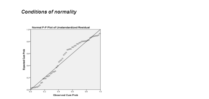
Figure 2 above shows that the scatter of the points are not random, indicating a lack of independence with no constant variance. Despite the above, there appears to be no outliers and thus an indication that the assumptions of the regression line were met. The implication is that no normality problems were identified.

Table 1 above indicates that the dependent and independent variables highly correlate and thus it can be said that there exists a negative relationship between the two variables. The Pearson correlation value of -0.845 is closer to -1 than it is to 0 and thus there is a strong negative linear relationship between defects and time period, and thus the analysis of the regression model can be continued.

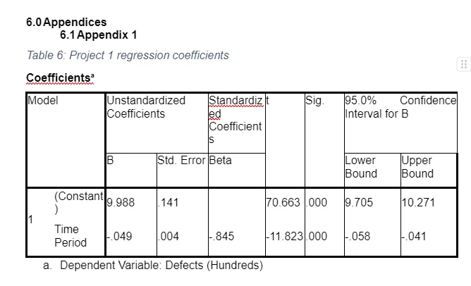
The model for stage one was as follows (See Table 6 in Appendix 1 for the coefficients); Defects (Hundreds) = 9.988 – 0.049 (Time Period) + 0.53130 Based on Table 2, time period significantly reduces the defects (increasing time period by one unit decreases defects by 0.049 units) [F(57, 1) = 139.783, p = .0001], R square = 0.714 (71.4%) and Adjusted R square = .709 (70.9%). That is, the model was statistically in determining the effectives of the defects reduction program with time period variations affecting 70.9% of the variations in defects.

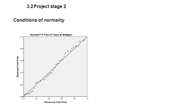
Figure 3 above indicates that points are distributed normally along the linear regression line indicating independence and a constant variance implying that the conditions of normality are met.

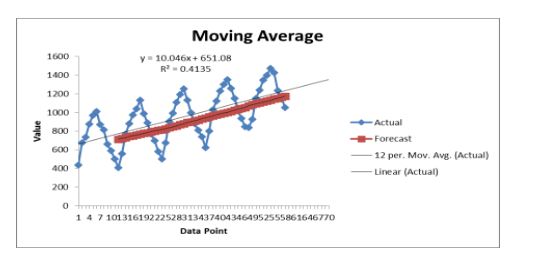
Table 3 above shows that only years in education and college GPA score have a correlation value of more than 0.5. All other variables are weak as regards to the correlation which implies that no problems of auto-correlated variables were identified. That is, the problem of auto-correlated variables exists where the independent variables show high correlation values (.9 and above; close to 1) (Székely and Bakirov, 2007). That is, the correlation between the various independent variables used is extremely high. This is an indication that the variables could be used as they are to produce the regression model.

The model insignificantly predicted the influence of the independent variables mentioned above on staff retention [F(39, 3) = 2.121, p = .115], R square = .15 (15%) and Adjusted R square = 0.079 (7.9%). The model is also not a good fit because, based on the R values, only 15% of the variations in years in education, age, and average college grade explain the variations in staff retention. Given the above, the insignificant variable (Years in Education) was removed from the model to develop and implement another multiple regression analysis models of two independent variables (College GPA Score and Age).

Model 2

It was found out that College GPA Score and Age significantly influenced staff retention [F(39, 2) = 3.248, p = .050], R square = .15 and Adjusted R square = .11. At F = 3.248 and p = .050, the null hypothesis is rejected concluding that there exists enough evidence that at least one of the variables of the multiple regression has a beta which is not equal to zero. Therefore, college average score and age are useful predictors of staff retention. Based on the model above, one unit increase in College GPA Score and Age increase Staff Retention value by 0.557 and 0.283 units respectively.

Discussion of the Results
Project stage 1

In summary, the results of the analysis in project stage 1 were significant, the models were relevant, and the variables used were useful. The analysis indicated that the last predicted value of defects (forecast) was 624, above the limit of 250. Therefore, the model significantly explained how defects are reducing as the program is being implemented. That is, based on the statistical analysis, as the program time period grows, the defects are reducing significantly implying that at one point in time they fall below 250 defects per month. Therefore, the suppliers did not meet their target.

Project stage

Even though the results were significant, the model was irrelevant to be used in solving the HR issues in the organisation because of a low R square value. That is, the data does not fit well into the model to provide statistically relevant results. This is among the various downsides of the model used in this stage. Therefore, the HR issues can be solved by considering high College GPA Scores and employee slightly older people than youth.

Benefits and downsides of the models used

The benefit of the models used for the two stages (1 and 2) is that they produced significant results with effectiveness and completeness. This is one of the advantages of linear models in that they can be used to effectively and completely analyse small data sets (Cohen, 2002). In these analyses, particularly in stage 1, it was clear that the models made effective use of the data provided. Despite the above, some models, like that of stage 2, were exposed to the problems of multicollinearity (the lack of independence between independent variables) which also led to poor extrapolation.

Based on the discussion above, the organisation is advised to use cubic or polynomial models which promote efficient extrapolation, reduce the problem of outliers, and normality and produce higher R square and significance values. Using these models, the organisation can develop effective models for forecasting.

Project stage 3

Regarding how the type of time series model to use was determined, as discussed in the research strategy, scatter plots in excel were developed which showed what types of models were being developed. The model fit was also considered which was determined by the use of the R square. Lastly, the error metric (MAPE) was used to achieve the goal under consideration. Therefore, multiplicative models with higher R square values and low MAPE values were deemed appropriate for use.

Figure 4 above shows the trend of the agricultural unit sales with the model being as follows: Agricultural Unit Sales = 10.046 (Time Period) + 651.08, R square = 0.4135 The model was used to forecast demand in future which follows a linear model (indicated in red in Figure 4) with the fitted values shown in Figure 5 below (the fitted values do not fit well within the model). Also, based on the scatter plot below, it is clear that the model is multiplicative.

Figure 6 above shows the trend of the industrial unit sales with the model being as follows: Industrial Unit Sales = 16.318 (Time Period) + 13720.2, R square = 0.6343 The model was also used to forecast demand in future which follows a linear model (indicated in red in Figure 6) with the fitted values shown in Figure 7 below (just like

in the first model above, the fitted values do not fit well within the model). Also, based on Figure 7 below, it is clear that the model is multiplicative.

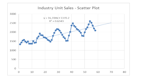
Based on the analysis above, the second model (for industry unit sales) is the best for use because it produces a higher R square value and a low MAPE. The indication is that the industry model is more accurate than the agricultural model, although both are multiplicative.

Regression results for the two sets of data (unit production costs) in stage 3 Model 1

Using the model Agricultural Unit Production Costs = 624.777 + 2.382 (Time Period) + 15.925, it can be said that, as time moves, the unit costs are increasing (See Appendix 3 Table 9). It should be noted that the significance of the model could not be identified in that there appear to be data problems in excel (See Appendix 3 Table 9 for F-tests and p-values). Despite the above, the usefulness of the model can be determined using the R square, which was 86.43% and MAPE = 2.58%.

Model 2

Using the model Industrial Unit Production Costs = 1779.381 + 6.029 (Time Period) + 25.235, it can also be stated that, as time moves, the industrial unit costs are increasing (See Appendix 3 Table 10). Just like in model 1, It should be noted that the significance of this model could not be identified as well, in that there appear to be data problems in excel (See Appendix 3 Table 10 for F-tests and p-values). Despite the above, the usefulness of the model can also be determined using the R square, which was 94.21% and MAPE = 1.45%.

Based on the analysis of the two models above, the second model (for industry costs) appears to be the best and most accurate in determining unit costs trends. This is so because it has higher R square and MAPE values as compared to that of model 1. This recommendation proves that the models used in this stage were beneficial and relevant in addressing the problems/issues in project stage 3.

Bibliography

• Cohen, J. C. P. W. S. &. A. L., 2002. Applied multiple regression/correlation analysis for the behavioral sciences. 3rd ed. s.l.: Psychology Press.
• Cramer, D., 2003. Advanced Quantitative Data Analysis. England: Open University Press.
• Dorey, F. J., 2011. In Brief: Statistics in Brief: Statistical Power: What Is It and When Should It Be Used?. Clinical Orthopaedics and Related Research, 469(2), p. 619–620.
• Field, A., 2013. Discovering Statistics using IBM SPSS Statistics. 4th ed. s.l.: Sage Publications Ltd.
• Hilbe, J. M., 2014. Modeling Count Data. s.l.:Cambridge University Press.
• Jarman, K. H., 2013. The Art of Data Analysis: How to Answer Almost Any Question Using Basic Statistics. New Jersey: John Wiley & Sons.
• Michiel, H., ed., 2001. Correlation (in statistics). In: Encyclopedia of Mathematics. s.l.: Springer.
• Székely, G. J. R. & Bakirov, N. K., 2007. Measuring and testing independence by correlation of distances. Annals of Statistics, 35(6), p. 2769–2794.

Take a deeper dive into Data Analysis And Interpretation with our additional resources.